Tutorial 7 – Torque Driven Treatment Optimization

Tutorial Developers: Robert Salati and B.J. Fregly, Rice Computational Neuromechanics Lab, Rice University

Last Updated: 11/4/2025

The Treatment Optimization toolset generates predictive simulations of a patient’s post-treatment movement function by optimizing specified treatment design parameters. The toolset consists of three tools designed using a “theme and variation” approach, where the tools are intended to be used in a specific order, with each tool serving a distinct purpose. Each tool uses the GPOPS-II direct collocation optimal control software for MATLAB and maintains a consistent structure for data inputs, problem design, cost function terms, constraint terms, and outputs, with variations.

This first section of the treatment optimization tutorial will cover the process of running Tracking Optimization (TO), Verification Optimization (VO), and Design Optimization (DO) in which joints are controlled by individual torque actuators. It will work through the design of settings files for all tools, along with analyzing the outputs of each tool with iterative problem-solving methods to generate good solutions.

The model used for this tutorial is the RCNL2024.osim model with the pelvis chosen as the root segment (i.e., the segment that connects the model to ground). All segments are kept in the model and the reference motion is three-dimensional, but only the right hip flexion, knee angle, and ankle angle motions are allowed to change. Limiting the predicted motion to the sagittal plane of only the kicking leg significantly reduces computation time for tutorial purposes.

Since we use repeated inverse dynamics analyses to generate predictive simulations, the root segment in the model will have unrealistic residual forces and torques acting on it. For the kicking model, root segment residual loads will therefore be present on the pelvis. If the model and data were perfect, these residual loads would be zero during the first 0.13 seconds of Tracking Optimization since both feet are off the ground in that time window.

For each predictive simulation, the motion of each generalized coordinate in the model is either:

1. Predicted (i.e., trajectory changeable as a function of time) or
2. Prescribed (i.e., trajectory pre-defined as a function of time).

If the coordinate name is included in the <states_coordinate_list> field, then motion of the coordinate will be predicted. If the coordinate name is not included in the <states_coordinate_list> field, then motion of the coordinate will be prescribed directly from the inverse kinematics data found in the <tracked_quantities_directory>.

For each generalized coordinate whose motion is predicted, if the coordinate name is also listed in the <RCNLTorqueController> field, then a force or torque controller is created to control that coordinate. For consistency with forces and torques calculated by inverse dynamics, the user should also add a <kinetic_consistency> constraint to ensure that the force or torque produced by the controller closely matches the corresponding force or torque calculated via inverse dynamics using the predicted motion and loads. Note, however, that a generalized coordinate can also have its motion predicted without having an associated torque controller.

Whether or not a torque controller should be created for a generalized coordinate depends on how the motion of the coordinate will be predicted. Generalized coordinate motion can be predicted by either:

1. Tracking a reference coordinate motion,
2. Tracking (or minimizing) a reference coordinate load (i.e., a control torque or inverse dynamics load), or
3. Tracking both a reference coordinate motion and a reference coordinate load simultaneously.

For Tracking Optimizations, both a reference coordinate motion and a reference coordinate load should be tracked simultaneously for each predicted coordinate, thereby producing dynamically consistent simulations that closely reproduce both inverse kinematics and inverse dynamics data simultaneously (i.e., spread out errors). Thus, both motion and load can be tracked simultaneously for the same coordinate during Tracking Optimizations. In contrast, for Verification and Design Optimizations, either motion or load should be tracked for the same coordinate. Thus, after Tracking Optimization is completed, the user should make a choice about how the motion of each generalized coordinate should be predicted, and then either track the reference coordinate motion (no <RCNLTorqueController> needed) or track/minimize the reference coordinate load (<RCNLTorqueController> required).

Section 1: Tracking Optimization

The Tracking Optimization (TO) tool uses a personalized model to produce a dynamically consistent movement simulation that closely reproduces all available experimental motion data, including joint motions, joint moments, ground reaction forces and moments, and muscle activations. To achieve a dynamically consistent motion, the tool spreads out matching errors between the different experimental quantities based on user-specified maximum allowable errors.

The tool accepts a post-JMP OpenSim model (.osim file) and personalized NMSM Pipeline model (.osimx fle) along with experimental inverse kinematics (IK) motions, inverse dynamics (ID) loads, ground reaction forces and moments, muscle–tendon lengths and velocities, muscle moment arms, and, if using synergy controls, NCP results for the trial of interest. This section of the tutorial will only be using torque controls with no external forces, so the only inputs we will use are a post-JMP OpenSim model, experimental IK motions, and experimental ID loads.

Before running Tracking Optimization:

1. Open the OpenSim model KickingModel.osim in the OpenSim GUI.

2. This model is a full three-dimensional gait model, but similar to the model personalization tutorials, this tutorial will only be using the right hip flexion, knee angle, and ankle angle coordinates.

3. This model uses a ground-pelvis joint, so inverse dynamics will yield unrealistic “residual” loads applied to the pelvis body.

4. With the model open in OpenSim, load the pre-calculated IK results in preprocessed\IKData\drive_kick1.sto to visualize the motion.

Creating a Tracking Optimization settings file:

1. Activate the NMSM GUI in OpenSim by navigating to Tools>User Plugins, and click rcnlPlugin.dll

2. With KickingModel.osim selected in the OpenSim GUI, navigate to Tools>Treatment Optimization>Tracking Optimization

   a. The following window should be opened:

   

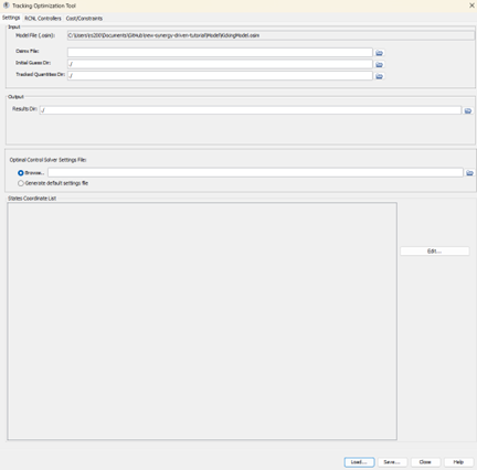
3. Leave the Osimx file field empty.

info

An input OsimX file would be used if we wanted external loads or muscles to be used in the TO, but this run will not use either.

4. Set the initial guess directory to preprocessed

5. Set the tracked quantities directory to preprocessed

6. Set the results directory to TorqueTOResultsV1

7. Set the optimal control solver settings file to gpopsSettings.xml

8. Under states coordinate list, select hip_flexion_r, knee_angle_r, ankle_angle_r

   a. The states coordinate list specifies which coordinates the optimizer is allowed to change. If a coordinate is not included in the states coordinate list, it is automatically prescribed. Therefore, most of the coordinates in this tutorial are prescribed.

9. Click on the RCNL Controllers tab at the top.

10. Under RCNL Torque Controller, add hip_flexion_r, knee_angle_r, ankle_angle_r to the coordinate list.

    a. These selections create individual torque actuators for each of the coordinates that we include in the states.

11. Click on the Cost/Constraints tab at the top.

tip

Tip for the upcoming section: When you click on the GUI drop down arrows to select cost term type, you can type the name of the cost term and the GUI will auto-navigate to the correct cost term.

12. Cost terms:

    a. Add a new cost term:

    - Name: Coordinate tracking
    - Cost: term type: generalized_coordinate_tracking
    - Component: list: (hip_flexion_r knee_angle_r ankle_angle_r)
    - Max: allowable error: 0.0873

    b. Add a new cost term:

    - Name: Speed tracking
    - Cost: term type: generalized_speed_tracking
    - Component: list: (hip_flexion_r knee_angle_r ankle_angle_r)
    - Max: allowable error: 0.873

    c. Add a new cost term:

    - Name: Load tracking
    - Cost: term type: inverse_dynamics_load_tracking
    - Component: list: (hip_flexion_r_moment knee_angle_r_moment ankle_angle_r_moment)
    - Max: allowable error: 50

13. Constraint terms:

    a. Add a new constraint term:

    - Name: Kinetic consistency
    - Constraint term type: kinetic_consistency
    - Component: list: (hip_flexion_r_moment knee_angle_r_moment ankle_angle_r_moment)
    - Max: error: 0.1
    - Min error: -0.1

14. Save this settings file as TorqueTOSettingsV1.xml

15. Open TorqueTOSettingsV1.xml in a text editor of your choice and explore it.

16. Change the <trial_name> field to be drive_kick1

Running Tracking Optimization:

1. Open MATLAB and open runTOTool.m in your tutorial directory.

2. Open the project file Project.prj inside your installation of nmsm-core.

3. Run the section labelled Run Torque TO V1

Post TO Analysis:

1. The script will create 4 plots for you:

   Plot 1 – Joint Angles: Joint angles for all model coordinates (including prescribed) as output by the TO run.

   Plot 2 – Joint Velocities: Joint velocities for all states coordinates.

   Plot 3 – Joint Loads: Joint loads for all model coordinates.

   Plot 4 – Torque Controls: Torque controls for all coordinates actuated by a torque controller.

2. These plots are a valuable way to analyze the results of the TO run. RMSE values between the tracked data and the TO results are reported for every plot where applicable.

3. It is also valuable to visualize the motion in the OpenSim GUI

   a. With the model selected in OpenSim, load the newly created IK motion in your TO results directory. Ensure the motion looks as close to the experimental motion as possible.

4. Getting a good TO run is hard and often requires additional iteration after the first attempt. It is recommended to add/remove cost terms if you believe the problem would benefit, or change max allowable errors for cost terms to “nudge” the solution in a desired direction.

Tracking Optimization with residual reduction:

1. One key function of the Tracking Optimization tool is to ensure dynamic consistency by reducing ground-pelvis residual loads to zero.

2. This model does not have external force data, so residual loads when the left foot is in contact with the ground are to be expected.

3. When both feet are out of contact with the ground at the start of the motion, there should be no residual loads acting on the pelvis.

4. In the NMSM OpenSim GUI, load TorqueTOSettingsV1

5. Change the results directory to TorqueTOSettingsV2

6. Set the states coordinate list to hip_flexion_r knee_angle_r ankle_angle_r hip_flexion_l knee_angle_l ankle_angle_l pelvis_tilt pelvis_tx pelvis_ty lumbar_extension arm_flex_r arm_flex_l

7. Add a new constraint term:

   - Name: Residual load reduction
   - Constraint term type: root_segment_residual_load
   - Component list: pelvis_tilt_moment, pelvis_tx_force, pelvis_ty_force
   - Max error: 1
   - Min error: -1

8. Save this settings file as TorqueTOSettingsV2

9. Open TorqueTOSettingsV2 in a text editor of your choice

10. Inside your <RCNLConstraintTerm> for Residual load reduction, copy and paste:

    <time_ranges>0 0.41</time_ranges>
    info

    Time ranges make the constraint only apply in between the given time points. The time range is in units of normalized time (0 to 1), and 0.41 in normalized time is equivalent to 0.31 seconds for this problem. In this case, the constraint is only applied while the model has no contact with the ground.

11. Run the MATLAB section labelled Run Torque TO V2

12. If we allow more coordinates to change, the optimizer can make small changes to get rid of any residual forces for a given time range.

13. This optimization takes longer, so for the remainder of the tutorial, we will be using the original set of states with no residual reduction.

Section 2: Verification Optimization

The Verification Optimization tool is used to perform a “dry run” Design Optimization without including any design elements, the goal being to ensure a good initial guess and to verify the appropriateness of the optimal control problem formulation. The tool accepts the same inputs as the TO tool, but in general, the results directory of a TO run is used for both the initial guess and tracked quantities.

The VO process will include two separate VO runs. The first run is essentially a “sanity check” and simply tracks the controls created by a previous TO run to verify that you get the same solution back. The second VO run is intended to by a dry run your DO problem formulation by adding in constraints that should be immediately satisfied to ensure that they are consistent with the rest of the problem formulation. If everything is consistent, both VO runs should converge very quickly to nearly identical solutions.

Creating a Verification Optimization settings file:

This section will walk you through the creation of a basic “sanity check” VO run.

1. Activate the NMSM GUI in OpenSim by navigating to Tools>User Plugins, and click rcnlPlugin.dll

2. With KickingModel.osim selected in the OpenSim GUI, go to Tools>Treatment Optimization>Verification Optimization

   a. A window should open that looks very similar to the Tracking Optimization window shown in section 1.

3. Leave the Osimx file field empty.

4. Set the initial guess directory to TorqueTOResultsV1

5. Set the tracked quantities directory to TorqueTOResultsV1

6. Set the results directory to TorqueVOResultsV1

7. Set the optimal control solver settings file to GpopsSettings.xml.

8. Under states coordinate list, select hip_flexion_r, knee_angle_r, ankle_angle_r

9. Click on the RCNL Controllers tab at the top.

10. Under RCNL Torque Controller, add hip_flexion_r, knee_angle_r, ankle_angle_r to the coordinate list.

11. Click on the Cost/Constraints tab at the top.

12. Cost terms:

    a. Add a new cost term:

    - Name: Controller tracking
    - Cost term type: controller_tracking
    - Component list: (hip_flexion_r knee_angle_r ankle_angle_r)
    - Max allowable error: 50

13. Constraint terms:

    a. Add a new constraint term:

    - Name: Kinetic consistency
    - Constraint term type: kinetic_consistency
    - Component list: (hip_flexion_r_moment knee_angle_r_moment ankle_angle_r_moment)
    - Max error: 0.1
    - Min error: -0.1

14. Save this settings file as TorqueVOSettingsV1.xml

15. Open TorqueVOSettingsV1.xml in a text editor of your choice and explore it. How does this settings file compare to your TO settings file?

16. Change the <trial_name> field to be drive_kick1

Running Verification Optimization:

1. Open MATLAB and open runVOTool.m in your tutorial directory.

2. Open the project file Project.prj inside your installation of nmsm-core.

3. Run the MATLAB section labelled Run Torque Driven VO V1.

Post VO Analysis:

1. The script will create the same 4 plots as the TO run.

2. The VO solution should be nearly identical to the TO solution. If there are large differences, there is likely a problem with your VO problem formulation.

Adding new constraints into VO:

The next step is to add constraints on top of our previous VO run to ensure that the constraints are consistent with your subsequent Desing Optimization problem formulation.

1. Load TorqueVOSettingsV1.xml into the VO NMSM OpenSim GUI.

2. Change the results directory to TorqueVOResultsV2.

3. Click to the Cost/Constraints tab at the top.

4. Constraint terms:

   a. Add a new constraint term:

   - Name: Initial coordinate position deviation
   - Constraint term type: initial_generalized_coordinate_deviation
   - Component list: hip_flexion_r, knee_angle_r, ankle_angle_r
   - Max error: 0.0175
   - Min error: -0.0175

   b. Add a new constraint term:

   - Name: Initial coordinate speed deviation
   - Constraint term type: initial_generalized_speed_deviation
   - Component list: hip_flexion_r, knee_angle_r, ankle_angle_r
   - Max error: 0.175
   - Min error: -0.175

   c. Add a new constraint term:

   - Name: Final toe marker position deviation
   - Constraint term type: final_marker_position_deviation
   - Component list: R_Toe
   - Max error: 0.001
   - Min error: -0.001

   d. Add a new constraint term:

   - Name: Final calcaneus orientation deviation
   - Constraint term type: final_body_orientation_deviation
   - Component list: calcn_r
   - Max error: 0.0175
   - Min error: -0.0175

   e. Add a new constraint term:

   - Name: Toe marker final velocity
   - Constraint term type: final_marker_velocity_value
   - Component list: R_Toe
   - Max error: 13.2
   - Min error: 13.1

5. Save this settings file as TorqueVOSettingsV2.xml

6. Open TorqueVOSettingsV2.xml in a text editor of your choice.

7. Inside your <RCNLConstraintTerm> for Toe marker final velocity, change <axes> to only include X.

   It is very important that <axes> only includes 'x', or your VO will not converge.

8. Run the MATLAB section labelled Run Torque Driven VO V2.

9. To compare both VO results to the previous TO results, run the MATLAB section labelled Compare Results. Both solutions should be near identical to the TO results

Section 3: Design Optimization

The Design Optimization tool predicts or optimizes how a planned treatment will affect a patient’s post-treatment movement function. The tool accepts the same inputs as the other Treatment Optimization tools, but typically VO results are used as the initial guess. Similar to VO, DO allows for controller tracking and generalized coordinate tracking alongside other DO-specific cost function terms.

Unlike the other Treatment Optimization tools, the DO tool allows for both fixed and free final time problem formulations. For free final time problems, the time vector can be constrained to a user defined range and tracked control quantities are stretched or compressed in time to match the current time vector. In addition to all cost function and constraint terms available in the TO and VO tools, the DO tool includes a number of additional built-in cost function terms.

Three key features of the DO tool are support for model modification functions, user-defined cost function terms, and user-defined constraint terms. By employing model modification functions alongside GPOPS-II’s static parameters feature, users can change the OpenSim musculoskeletal model, modify the neural control model, or adjust parameter values in an assistive device. Creating a Design Optimization settings file:

Now that we have a good “dry run” VO run, we can incorporate some design aspects into our treatment optimization. This will be an iterative process, so first we will create a “base” DO settings file that we will build upon for subsequent runs.

1. Activate the NMSM GUI in OpenSim by navigating to Tools>User Plugins, and click rcnlPlugin.dll

2. With KickingModel.osim selected in the OpenSim GUI, Tools>Treatment Optimization>Design Optimization

a. A window should open that looks very similar to the Tracking Optimization window shown in section 1.

3. Leave the Osimx file field empty.

4. Set the initial guess directory to TorqueVOResultsV2

5. Set the tracked quantities directory to TorqueVOResultsV2

6. Set the results directory to TorqueDOResultsV1

7. Set the optimal control solver settings file to gpopsSettings.xml.

8. Under states coordinate list, select hip_flexion_r, knee_angle_r, ankle_angle_r

9. Click on the RCNL Controllers tab at the top.

10. Under RCNL Torque Controller, add hip_flexion_r, knee_angle_r, ankle_angle_r to the coordinate list.

11. Click on the Cost/Constraints tab at the top.

    a. The below steps are using the exact same cost terms and constraints as in TorqueVOSettingsV2.xml. To save time, you may save the settings file right now as TorqueDOSettingsV1.xml and copy the <RCNLCostTermSet> and <RCNLConstraintTermSet> from TorqueVOSettingsV2.xml over to TorqueDOSettingsV1.xml. If copying from past settings files, skip to bullet point 15.

12. Cost terms:

    a. Add a new cost term:

    - Name: Controller tracking
    - Cost term type: controller _tracking
    - Component list: hip_flexion_r knee_angle_r ankle_angle_r
    - Max allowable error: 25

13. Constraint terms:

    a. Add a new constraint term:

    - Name: Kinetic consistency
    - Constraint term type: kinetic_consistency
    - Component list: (hip_flexion_r_moment knee_angle_r_moment ankle_angle_r_moment)
    - Max error: 0.1
    - Min error: -0.1

    b. Add a new constraint term:

    - Name: Initial coordinate position deviation
    - Constraint term type: initial_generalized_coordinate_deviation
    - Component list: hip_flexion_r knee_angle_r ankle_angle_r
    - Max error: 0.0175
    - Min error: -0.0175

    c. Add a new constraint term:

    - Name: Initial coordinate speed deviation
    - Constraint term type: initial_generalized_speed_deviation
    - Component list: hip_flexion_r knee_angle_r ankle_angle_r
    - Max error: 0.175
    - Min error: -0.175

    d. Add a new constraint term:

    - Name: Final toe marker position deviation
    - Constraint term type: final_marker_position_deviation
    - Component list: R_Toe
    - Max error: 0.001
    - Min error: -0.001

    e. Add a new constraint term:

    - Name: Final calcaneus orientation deviation
    - Constraint term type: final_body_orientation_deviation
    - Component list: calcn_r
    - Max error: 0.0175
    - Min error: -0.0175

    f. Add a new constraint term:

    - Name: Toe marker final velocity
    - Constraint term type: final_marker_velocity_value
    - Component list: R_Toe
    - Max error: 14.4
    - Min error: 14.3

14. Save this settings file as TorqueDOSettingsV1.xml

a. This will be the base settings file that we iterate out of later.

15. Open TorqueDOSettingsV1.xml in a text editor of your choice and explore it.

16. Change the <trial_name> field to be drive_kick1

17. Inside your <RCNLConstraintTerm> for Toe marker final velocity, change <axes> to only include X, and change the <max_error> to 14.4 and <min_error> to 14.3 if not already done.

18. Open MATLAB and open runDOTool.m in your tutorial directory.

19. Open the project file Project.prj inside your installation of nmsm-core.

20. Run the MATLAB section labeled Run Torque DO V1.

Iterate through DO formulations:

Iteration 1:

1. If everything up to now was done correctly, the DO problem should converge to a solution that “flicks” the ankle angle forward to increase the final toe marker velocity. This solution is valid and satisfies the given problem constraints, but is not a realistic representation of how soccer players actually kick a soccer ball. Typically, the players ankle is locked, and kicking power comes from the hip and knee.

2. To move the solution towards a more realistic motion, we can add more constraints to impose certain behaviors. In this case, we can limit the ankle motion in our solution.

3. Open TorqueDOSettingsV1.xml in the NMSM OpenSim GUI

4. Change the results directory to TorqueDOSettingsV2

5. Constraint terms:

   a. Add a new constraint term:

   - Name: Limit ankle position bounds
   - Constraint term type: generalized_coordinate_value
   - Component list: ankle_angle_r
   - Max error: 0.0475
   - Min error: -0.3187

   b. Add a new constraint term:

   - Name: Limit ankle velocity path
   - Constraint term type: generalized_speed_deviation
   - Component list: ankle_angle_r
   - Max error: 0.175
   - Min error: -0.175

6. Save this settings file as TorqueDOSettingsV2.xml.

7. Run the MATLAB section labeled Run Torque DO V2.

8. Note that the knee and hip have larger changes now.

Iteration 2:

1. Design optimization includes the option for “free final time” problems, in which the final time of the simulation is a variable that can be changed.

2. Free final time is important for a problem such as speeding up a soccer kick, because the new motion might become longer or shorter than the experimental motion because of kinematic changes.

3. Create a copy of TorqueDOSettingsV2.xml and name it TorqueDOSettingsV3.xml

4. Open TorqueDOSettingsV3.xml in a text editor of your choice

5. Change <results_directory> to TorqueDOResultsV3

6. Underneath the <trial_name> field, copy and paste:

   <final_time_range>0.26 0.36</final_time_range>

a. This allows the solution’s final time to be anywhere between 0.26 and 0.36 seconds.

7. Run the MATLAB section labeled Run Torque DO V3

Iteration 3:

1. Increasing the final foot velocity can also be achieved using a user defined cost term.

2. A user defined cost term is premade in the tutorial directory named footSpeedCost.m

   a. This cost term minimizes deviations away from a desired final velocity.

3. Note: If you are using user defined cost terms, the NMSM GUI in OpenSim is not recommended. If you load a settings file with a user defined cost term into the GUI, and then save a new settings file, the user defined cost term will not be saved properly.

4. Copy your TorqueDOSettingsV3.xml and rename the new settings file TorqueDOSettingsV4.xml

5. Change the results directory to TorqueDOResultsV4.

6. To include this cost term in the settings file, copy the following lines into your <RCNLCostTermSet>

   <RCNLCostTerm name="User defined">
       <type>user_defined</type>
       <function_name>footSpeedCost</function_name>
       <cost_term_type>discrete</cost_term_type>
       <is_enabled>true</is_enabled>
       <marker_name>R_Toe</marker_name>
       <target_speed>14.35</target_speed>
   </RCNLCostTerm>

7. Inside your <RCNLConstraintTerm> for Toe marker final velocity, set <is_enabled> to false

8. Run the MATLAB section labeled Run Torque DO V4.

Iteration 4:

1. Just like we have user defined cost terms, we can also create user a defined constraint term.

2. Next, we will use a pre-made user defined constraint term that increases the kick speed.

3. We already have a constraint term that increases the toe marker velocity, so we will recreate that same constraint in the user defined framework for demonstration. This constraint term is in footSpeedConstraint.m

4. Copy your TorqueDOSettingsV3.xml and rename the new settings file TorqueDOSettingsV5.xml

5. Change the results directory to TorqueDOResultsV5.

6. To include this constraint term in the settings file, copy the following lines into your <RCNLConstraintTermSet>

   <RCNLConstraintTerm name="Toe marker final velocity">
       <is_enabled>true</is_enabled>
       <!--Type of constraint term.-->
       <type>user_defined</type>
       <!--Type of application of constraint term (path or terminal).-->
       <constraint_term_type>terminal</constraint_term_type>
       <!--Name of Matlab function defining constraint term.-->
       <function_name>footSpeedConstraint</function_name>
       <marker_name>R_Toe</marker_name>
       <!--Maximum error allowed by this constraint term.-->
       <max_error>14.4</max_error>
       <!--Minimum error allowed by this constraint term.-->
       <min_error>14.3</min_error>
   </RCNLConstraintTerm>

7. Inside your <RCNLConstraintTerm> for Toe marker final velocity, set <is_enabled> to false

8. Run the MATLAB section labeled Run Torque DO V5.

Post DO Analysis:

1. After running the four iterations on Torque Driven Design Optimization, we can plot results against each other to compare.

2. Run the section titled Compare Results and compare the results from iteration 3 (using a constraint on the final toe marker velocity), iteration 4 (using a user defined cost term), and iteration 5 (using a user defined constraint term)

3. All plots should look very similar, demonstrating that both methods arrived at similar solutions.

4. We see that most of the increase in speed is coming from the hip and knee as intended.