Tutorial 5 – Ground Contact Personalization

Tutorial Developers: Robert Salati, Spencer Williams, and B.J. Fregly, Rice Computational Neuromechanics Lab, Rice University

Last Updated: 11/4/2025

The Ground Contact Model Personalization tool finds physical properties for elastic foundation foot–ground contact models that closely reproduce experimental ground reaction forces and moments while allowing slight changes in foot kinematics. The elastic foundation is composed of a uniform grid of linear springs with nonlinear damping and friction placed across the bottom of the foot. A personalized foot-ground contact model is important for predicting new movements because ground reaction forces and moments will change with the new movements.

The inputs to the GCP tool are a post-JMP lower-body or full-body OpenSim model along with IK motion and associated ground reaction data for a walking trial, where the IK and ground reaction data must possess the same time increments.

Before running GCP:

1. Open the OpenSim model BodyModel.osim in the OpenSim GUI.

2. GCP uses the model’s default pose to place springs on the foot. It is important that this model has the feet flat on the ground and at the correct height above the ground. With these criteria, the static pose is generally a good choice for the default pose.

3. Run OpenSim Inverse Kinematics on BodyModel.osim with the premade settings file IKSettingsStaticPose.xml.

4. Click on the Coordinates tab

5. Under poses, click Set Default and save the model. The default model pose is now the static trial pose.

Setting up a GCP settings file:

1. Activate the NMSM GUI in OpenSim by navigating to Tools>User Plugins, and click rcnlPlugin.dll.

2. With bodyModel.osim selected in the OpenSim GUI, navigate to Tools>Model Personalization>Ground Contact Personalization.

   a. The following window should be opened:

   

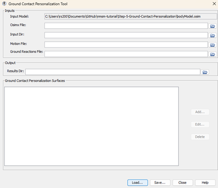
3. Leave the Osimx file field empty.

4. Choose the motion file to be preprocessed\IKData\gait_1.sto

5. Choose the ground reactions file to be preprocessed\GRFData\gait_1.sto

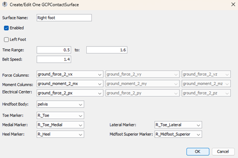
6. Choose the results directory to be GCPResultsV1

7. Add a new contact surface named Right Foot

8. Set the time range to 0.5 – 1.6

9. Set the belt speed to 1.4

10. Set the force columns to ground_force_2_vx ground_force_2_vy ground_force_2_vz

11. Set the moment columns to ground_moment_2_mx ground_moment_2_my ground_moment_2_mz

12. Set the electrical center columns to ground_force_2_px ground_force_2_py ground_force_2_pz

13. Set Hindfoot Body to calcn_r

    a. Tip: You can type inside the drop down menu to get to the option you want faster.

14. Set the markers as follows:

        - Toe Marker: R_Toe
        - Medial Marker: R_Toe_Medial
        - Heel Marker: R_Heel
        - Lateral Marker: R_Toe_Lateral
        - Midfoot Superior Marker: R_Midfoot_Superior

    Your full contact surface should look like the following:

    

15. Save your settings file as GCPSettingsV1.xml

16. Open up GCPSettingsV1.xml in a text editor of your choice and explore the settings file.

17. With a text editor, scroll to the bottom of the settings file, and change <max_iterations> to 20.

    a. This is to make the optimization terminate earlier to save time.

Running GCP:

1. Open MATLAB and open runGCP.m in your tutorial directory.

2. Open the project file Project.prj inside your installation of nmsm-core.

3. Ensure MATLAB is set up to use multi-processing, not multi-threading:

   a. In the bottom left of MATLAB, click the parallel processing icon, and click parallel preferences.

   b. In the drop down menu for Default Profile, select Processes.

4. Run the MATLAB section labelled Run GCP V1

   a. With the section selected, press control+enter to run a section.

5. While running GCP:

   a. In the OpenSim GUI, open and inspect the model footModel_1.osim

   b. To simplify the optimization, GCP only uses foot kinematics instead of full body kinematics.

   c. The location of the springs is determined by the default pose of the osim model. To place the springs well, it is important that the full body model’s feet are flat on the ground and placed at an appropriate height.

Post GCP analysis:

1. Look through the plots created by the script. If everything was done correctly, there should be 3 plots.

   Plot 1 – Ground Reaction Matching: Ground reaction forces and moments produced by the contact model plotted against experimental ground reactions.

   Plot 2 – Kinematics: Adjusted foot kinematics produced by the optimization.

   Plot 3 – Stiffness Coefficients: A grid of stiffness coefficients for each foot.

Experiment with electrical center adjustment:

1. Create a copy of GCPSettingsV1.xml and name it GCPSettingsV2.xml

2. Open GCPSettingsV2.xml in a text editor of your choice.

3. Change the <results_directory> to GCPResultsV2.

4. In task 3 of your <GCPTaskSet>, change <electricalCenterX> and <electricalCenterZ> to true.

5. Save this settings file as GCPSettingsV2.xml

6. Run the MATLAB section labelled Run GCP V2

   a. With the section selected, press control+enter to run a section.

Experiment with viscous friction:

1. Create a copy of GCPSettingsV1.xml and name it GCPSettingsV3.xml

2. Open GCPSettingsV3.xml in a text editor of your choice.

3. Change the <results_directory> to GCPResultsV3.

4. In all tasks, set <dynamicFrictionCoefficient> to false, and <viscousFrictionCoefficient> to true.

5. At the bottom of the settings file, set <initial_dynamic_friction_coefficient> to 0, and <initial_viscous_friction_coefficient> to 5.

6. Save this settings file as GCPSettingsV3.xml

7. Run the MATLAB section labelled Run GCP V3

   a. With the section selected, press control+enter to run a section.

Experiment with grid density:

1. Create a copy of GCPSettingsV1.xml and name it GCPSettingsV4.xml

2. Open GCPSettingsV4.xml in a text editor of your choice.

3. Change the <results_directory> to GCPResultsV4.

4. At the top of the file, set <grid_width> to 8, and <grid_height> to 15.

5. Save this settings file as GCPSettingsV4.xml

6. Run the MATLAB section labelled Run GCP V4

   a. With the section selected, press control+enter to run a section.