MODULE 3: SYNERGY-DRIVEN TRACKING OPTIMIZATION
In this module, you will use the NMSM Pipeline Tracking Optimization tool with your personalized skeletal geometry and neural control model to create a dynamically consistent synergy driven walking simulation that closely reproduces experimental joint motion, joint moment, ground reaction, and EMG data. Tracking Optimization results always provide the starting point for the NMSM Pipeline Treatment Optimization Process. In the subsequent module, you will perform a Verification Optimization (VO) starting from your TO results to confirm that your TO results are reliable, followed by a Design Optimization (DO) to design a synergy-based FES treatment for our stroke subject.
Similar to module 2, synergy-driven TO problems can take a long time to run, and so this project will focus more on analysis of synergy-driven TO results rather than on running multiple iterations of TO. You will only do one synergy-driven TO run, where the focus is primarily on getting the optimization to converge, not on getting an optimal result. A results directory with final results will be provided as a part of the assignment for analysis.
Synergy-driven TO problems are formulated similarly to torque-driven TO problems, but are generally much harder for the optimal control solver to find a solution. This difficulty arises because actuating a model with muscles is more complicated than discrete torque actuators on muscle joints. The additional problem complexity means that Synergy-driven TO is very sensitive to the input data it is given. If the prerequisite model personalization was not high quality, synergy-driven TO will often struggle to converge on a good solution. However, if effort is put out to get good quality and anatomically correct model personalization results, synergy-driven TO can converge quickly.
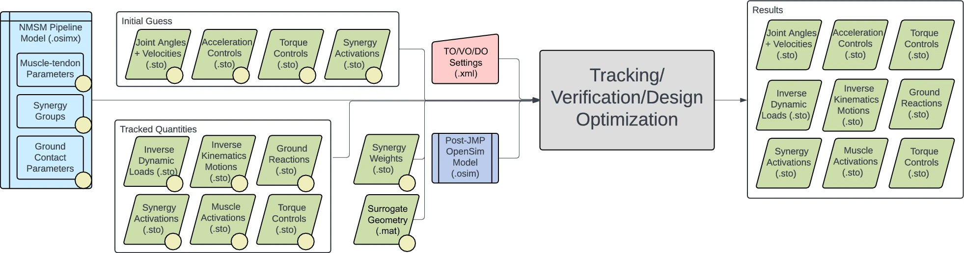
Synergy-driven TO makes use of input data from a variety of sources throughout the NMSM Pipeline. Firstly, you should always use a post-JMP OpenSim model. If your problem includes ground reactions, TO expects an osimx file containing a GCP contact surface set. Because synergy-driven TO uses muscle actuators, it requires both MTP results and NCP results. TO uses the calibrated muscle models from NCP and uses the muscle synergies calculated by NCP as an initial guess to calculate more dynamically consistent synergies. Finally, synergy-driven TO expects that your input data is formatted as prescribed by the preprocessing sub-tool. Therefore, you will be using the same preprocessing directory that you have used for the previous subprojects. The interaction between tool settings, data, and models required to perform this module is shown in the figure below:
Task 1: Surrogate Muscle Geometry
An important step before all synergy-driven Tracking Optimization runs is to create a surrogate muscle geometry model. As we explored briefly in module 1, muscle geometry calculations are computationally expensive. Running the muscle analysis tool with all 86 muscles in the RCNL2025 model can take minutes for just one gait cycle. This was not problematic for MTP and NCP because the motion was not being changed by those tools, and so muscle analysis only needed to be run once. For Treatment Optimization however, the motion changes every iteration, and so muscle geometry needs to be recalculated repeatedly. This quickly becomes a problem for generating walking simulations.
The solution to this problem is to create a surrogate muscle geometry model that allows for muscle geometry calculations to be done much quicker. Rather than running a full muscle analysis calculation multiple times, we can fit a 6th order polynomial to the muscle geometry as a function of modeled joint angles. In short, we can run muscle analysis on a gait cycle and fit the muscle-tendon lengths and muscle-moment arms to the modeled joint angles. This polynomial model allows us to quickly and easily calculate muscle moment arms for a given model orientation.
The next problem that arises is selecting the proper motions to fit a surrogate model with. If we only use gait data to fit a surrogate model, then any new motions that deviate from the original motion will incur errors in muscle moment arms. On the other hand, we don’t want to exhaustively sample every combination of model coordinates, because that will take far too much computation time to fit the surrogate model. The solution is to meet in the middle, and sample combinations of coordinates in the neighborhood around the original gait data. As such, the surrogate geometry uses a Latin hypercube sampling (LHS) algorithm to sample combinations of coordinates close to the original motion. LHS randomly searches combinations of coordinates using a minimal set of combinations that effectively covers the entire search space. We define the search space here to be the joint angles during gait motion ±20°.
Step 1: Create your surrogate kinematics
Open the Matlab script
surrogateKinematicsScript.minfoThis surrogate kinematics script samples joint angles in the area around the given gait data. Ideally, these sampled joint angles will encompass any new predicted motions and allow their moment arms to be accurate and quickly calculated.
Fill out the variables for
modelFileName, andreferenceKinematicsFile.inforeferenceKinematicsFileshould be your IK data inpreprocessing.Set angularPadding value to 20°
Set linearPadding to 0.1m.
infoThese variables adjust the sampling range around the base IK files. A larger value means you are sampling a wide range of joint coordinate values.
Click Run.
Start OpenSim and load
UF_Subject_4_Scaled_JMP.osimLoad the motion
surrogateData\IKData\gait_1.stoQuestionBriefly describe what is happening in this motion.
Expand for answer
The surrogate kinematics motion consists of the base gait motion with joints randomly sampled around that motion. The motion looks very noisy, but you might be able to see the base gait motion underneath all of the noise.
Step 2: Run muscle analysis
Open the Analyze tool in OpenSim.
Set your input motion to
surrogateData\IKData\gait_1.stoDo not filter this motion.The motion looks very noisy but that is by design. The surrogate kinematics script adds “noise” to the base motion so that the sampling area for moment arms is larger.
Set your Prefix to
gait_1Set your output directory to
surrogateData\MAData\gait_1Add a muscle analysis set
Click run.
RuntimeThis muscle analysis run will take about 20 minutes depending on computer speed.
You now have a set of muscle-tendon lengths and moment arms for every combination of joint angles produced in step 1. TO will automatically fit a polynomial to these values at the start of your run.
Task 2: Initial Tracking Optimization
This module task will focus on getting an initial guess synergy-driven Tracking Optimization. Because synergy-driven TO is such a complicated problem, one of the primary challenges in getting a good result is simply getting the optimal control problem to converge in the first place. A good method to get an initial TO to converge is to start the problem with very loose cost terms, and tight constraint terms. Once this loosely defined optimization converges, the next step is to progressively and systematically tighten cost terms and constraint terms until a satisfactory solution is obtained. This process allows us to diagnose if the constraint terms being used are compatible with each other, and systematically tightening the problem allows us to diagnose where the primary difficulties in convergence may come from.
Step 1: Create TO Settings File
- Load your post-JMP model
UF_Subject_4_Scaled_JMP.osiminto the OpenSim GUI - Open the Tracking Optimization GUI
- Set the Input Osimx File to be the Osimx file generated by your final NCP run
- Set the Tracked Quantities Directory to
Preprocessing\preprocessed - Set the Initial Guess Directory to your final NCP results directory
- Set the Trial Prefix to
gait_1 - Set the Results Directory to
TrackingOptimization\SynergyTOResultsV1 - Set the Optimal Control Settings File to
TrackingOptimization\gpopsSettings.xml - Add all unlocked coordinates to States Coordinates List.
- Go to the RCNL Controllers tab
- Keep Optimize Synergy Vectors disabled
- For the Coordinates List, select all unlocked lower limb coordinates
Unlike the torque controller coordinate list, the synergy controller coordinate list does not control which coordinates are controlled by the synergy controller.
This coordinate list controls which joints are included in the surrogate model. If a joint has muscles crossing it and is unlocked in your model, you want to include it in your surrogate model because that joint motion will affect muscle moment arms.
You should almost always include every unlocked joint that has muscles crossing it in the surrogate model coordinate, regardless of if you want those joints to be muscle controlled or not.
- Set the Surrogate Model Data Directory to
TrackingOptimization\surrogateData - Go to the Cost/Constraints tab
- Add the following cost and constraint terms:
Cost Terms
Name: Lower limb coordiante tracking loose
Type: generalized_coordinate_tracking
Components:
    hip_flexion_r
    knee_angle_r
    ankle_angle_r
    hip_flexion_l
    knee_angle_l
    ankle_angle_l
Max Allowable Error: 0.3
Name: Lower limb coordinate tracking tight
Type: generalized_coordinate_tracking
Components:
    hip_adduction_r
    hip_rotation_r
    subtalar_angle_r
    mtp_angle_r
    hip_adduction_l
    hip_rotation_l
    subtalar_angle_l
    mtp_angle_l
Max Allowable Error: 0.15
Name: Upper limb coordinate tracking loose
Type: generalized_coordinate_tracking
Components:
    lumbar_extension
    lumbar_bending
    lumbar_rotation
    arm_flex_r
    arm_add_r
    arm_rot_r
    elbow_flex_r
    arm_flex_l
    arm_add_l
    arm_rot_l
    elbow_flex_l
Max Allowable Error: 0.3
Name: Pelvis translation tracking
Type: generalized_coordinate_tracking
Components:
    pelvis_tx
    pelvis_tz
Max Allowable Error: 0.05
Why do we not track pelvis_ty?
Expand for answer
Name: Pelvis rotation tracking
Type: generalized_coordinate_tracking
Components:
    pelvis_tilt
    pelvis_list
    pelvis_rotation
Max Allowable Error: 0.15
Name: ID load tracking
Type: inverse_dynamics_load_tracking
Components:
    hip_flexion_r_moment
    hip_adduction_r_moment
    hip_rotation_r_moment
    knee_angle_r_moment
    ankle_angle_r_moment
    subtalar_angle_r_moment
    hip_flexion_l_moment
    hip_adduction_l_moment
    hip_rotation_l_moment
    knee_angle_l_moment
    ankle_angle_l_moment
    subtalar_angle_l_moment
Max Allowable Error: 25
Name: Speed tracking
Type: generalized_speed_tracking
Components:
    all unlocked coordinates
Max Allowable Error: 5
Name: Vertical external force tracking
Type: external_force_tracking
Components:
    ground_force_1_vy
    ground_force_2_vy
Max Allowable Error: 100
Name: Horizontal external force tracking
Type: external_force_tracking
Components:
    ground_force_1_vx
    ground_force_1_vz
    ground_force_2_vx
    ground_force_2_vz
Max Allowable Error: 25
Name: External moment tracking y z
Type: external_moment_tracking
Components:
    ground_moment_1_my
    ground_moment_1_mz
    ground_moment_2_my
    ground_moment_2_mz
Max Allowable Error: 20
Name: External moment tracking x
Type: external_moment_tracking
Components:
    ground_moment_1_mx
    ground_moment_2_mx
Max Allowable Error: 20
Name: Muscle activation tracking
Type: muscle_activation_tracking
Components:
    All model muscles
Max Allowable Error: 0.25
Name: Synergy activation tracking
Type: controller_tracking
Components:
    right_leg_1
    right_leg_2
    right_leg_3
    right_leg_4
    right_leg_5
    left_leg_1
    left_leg_2
    left_leg_3
    left_leg_4
    left_leg_5
Max Allowable Error: 0.5
Constraint Terms
Name: Kinetic consistency
Type: kinetic_consistency
Components:
    hip_flexion_r_moment
    hip_adduction_r_moment
    hip_rotation_r_moment
    knee_angle_r_moment
    ankle_angle_r_moment
    subtalar_angle_r_moment
    hip_flexion_l_moment
    hip_adduction_l_moment
    hip_rotation_l_moment
    knee_angle_l_moment
    ankle_angle_l_moment
    subtalar_angle_l_moment
Max/Min Error: 0.1/-0.1
Why don't we have kinetic consistency on the toe?
Name: Residual force reduction
Type: root_segment_residual_load
Components:
    pelvis_tx_force
    pelvis_ty_force
    pelvis_tz_force
Max/Min Error: 25/-25
Name: Residual moment reduction
Type: root_segment_residual_load
Components:
    pelvis_tilt_moment
    pelvis_list_moment
    pelvis_rotation_moment
Max/Min Error: 10/-10
For a full TO run, we typically have residual load reduction at 1/-1 for forces and 0.1/-0.1 for moments. These values are larger than that just to speed up convergence for tutorial purposes.
Name: Rotational coordinate periodicity
Type: generalized_coordinate_periodicity
Components:
    All rotational coordinates (not pelvis translation coordinates)
Max/Min Error: 0.01/-0.01
Name: Translational coordinate periodicity
Type: generalized_coordinate_periodicity
Components:
    pelvis_tx
    pelvis_ty
    pelvis_tz
Max/Min Error: 0.01/-0.01
Name: External force periodicity
Type: external_force_periodicity
Components:
    ground_force_2_vx
    ground_force_2_vy
    ground_force_2_vz
    ground_force_1_vx
    ground_force_1_vy
    ground_force_1_vz
Max/Min Error: 5/-5
Name: External moment periodicity
Type: external_moment_periodicity
Components:
    ground_moment_2_mx
    ground_moment_2_my
    ground_moment_2_mz
    ground_moment_1_mx
    ground_moment_1_my
    ground_moment_1_mz
Max/Min Error: 1/-1
Name: Rotational speed periodicity
Type: generalized_speed_periodicity
Components:
    All rotational coordinates (not pelvis translation coordinates)
Max/Min Error: 0.1/-0.1
Name: Translational speed periodicity
Type: generalized_speed_periodicity
Components:
    pelvis_tx
    pelvis_ty
    pelvis_tz
Max/Min Error: 0.01/-0.01
- Inside
gpopsSettings.xml, change<setup_nlp_max_iterations>to 250 - Inside your settings file, inside
<RCNLSynergyController>, copy and paste:
<load_surrogate_model>true</load_surrogate_model>
Fitting the surrogate model can take a long time for our model, so this line loads a preexisting surrogate model into the TO run to save time.
- Open the Matlab script
TrackingOptimization\runTO.mand click Run.
This TO run will take approximately 300 iterations to converge.
Step 1a: Analyze Convergence
This step should be done while your TO is running.
After clicking Run on Matlab, you will see a similar output to the following appear after about 10 minutes:
| iter | objective | inf_pr | inf_du | lg(mu) | ||d|| | lg(rg) | alpha_du | alpha_pr | ls |
|---|---|---|---|---|---|---|---|---|---|
| 0 | 9.1398349e-02 | 2.10e+03 | 6.14e-03 | 0.0 | 0.00e+00 | - | 0.00e+00 | 0.00e+00 | 0 |
| 1 | 9.1034505e-02 | 2.07e+03 | 4.22e+00 | -2.3 | 1.35e+00 | - | 9.98e-03 | 2.11e-02f | 1 |
| 2 | 9.1321351e-02 | 1.99e+03 | 2.52e+01 | -2.3 | 1.11e+00 | - | 1.21e-02 | 3.54e-02f | 1 |
| 3 | 9.3515725e-02 | 1.82e+03 | 1.19e+02 | -2.3 | 1.94e+00 | - | 2.23e-02 | 6.91e-02h | 1 |
The main important columns in this output are iter, objective, inf_pr, and inf_du. The objective column is the value for the cost function, where a lower value is a better adherence to the cost function. inf_pr and inf_du are the primal and dual infeasibility, respectively, and correspond to constraint satisfaction. Specifically, inf_pr corresponds to how well constraints are satisfied, and inf_pr corresponds to how well the cost function and constraint function agree with each other. If inf_pr is low (constraints are satisfied), but inf_du is high, that roughly means that the cost function could be lower than it currently is. In this case, the constraints might be satisfied, but the solution is not “optimal” because the cost function is still too high. The optimization is configured to converge when both inf_pr<9.99e-5 and inf_du<9.99e-1.
As mentioned earlier in the assignment, a key challenge in synergy-driven TO is simply getting the optimization to converge. The optimization you are running should take around 200 iterations to converge. During this time, if inf_pr>1.00e4 or inf_du>1e6 for more than 10 iterations, it is unlikely that your optimization will converge. To save time, you should stop the optimization and troubleshoot your settings file. Another sign that your optimization will likely not converge is if the letter “r” appears next to your iteration counter. This sign means that the optimizer entered “restoration” mode. Put simply, the optimizer found that the current search space was not feasible (meaning the constraints cannot be satisfied). While entering restoration mode does not always mean the optimization will not converge, it is typically good practice to cancel the optimization if it occurs because it is likely that the problem as a whole is not feasible.
Some likely problems that can cause an optimization to not converge are:
Data quality issues: This will likely not be a problem for this project but is important if you are doing your own research.
Conflicting constraint terms: If you have constraint terms with conditions that conflict with each other, the problem as a whole will be infeasible and inf_pr and inf_du will quickly increase.
Cost terms conflict with constraint terms: This often happens if cost terms are too tight and don’t give the optimizer freedom to satisfy constraints. Alternatively, if you include inappropriate cost terms, constraints will also be difficult to match. An example of this is tracking pelvis_ty in the cost function. This cost term will not work well with residual reduction, because tracking pelvis_ty forces the model into the ground which can increase the vertical residual force.
Other infeasible constraints: Often constraints are simply not able to be satisfied. For example, in the kicking tutorial, we increase the toe marker velocity by using a constraint term to force the X velocity of the toe marker to be 14.3-14.4 m/s. If however, you include the Y and Z velocities in that constraint terms, the problem will not converge because those velocities will not reasonably reach 14.3-14.4 m/s
Check your settings file for these issues, and if you still are not sure why your optimization is not converging, consider asking about it on the SimTK forum.
Step 2: Analyze Full TO Results
The previous section walked you through how to create an initial TO settings file. That TO should have converged, thereby demonstrating problem feasibility, but the settings still needed to be iterated on to get the best solution. Next, you can analyze a final TO run from the end of that iteration process.
In this run, cost and constraint terms were systematically tightened to yield an optimal solution. Another key change was that synergy vectors were optimized as well. We found that allowing small changes in synergy vectors is important for getting a good TO solution. To go along with changing the synergy vectors, we also track the NCP synergy vectors to make sure they don’t change too much.
In the TO run you did in step 1, synergy vectors were not optimized, meaning we effectively assumed that the synergy vectors created by NCP were perfect. While the synergy vectors created by NCP should be very close to the true synergy vectors, giving TO some freedom to change them often helps get a better solution. One drawback to allowing synergy vectors to change is that it slows down the optimization significantly.
To view the settings file used to get these results, you may open SynergyTOResultsFull\TOSettings.xml. You can plot these TO results compared to your initial TO results by uncommenting the code on line 7 inside runTO.m.
Deliverables
In 1-2 sentences, describe the goal of Tracking Optimization
Why is synergy-driven tracking optimization generally harder than torque-driven tracking optimization? Give 2 reasons.
What is the main reason we want to use a surrogate muscle geometry model?
Briefly describe the process for creating a surrogate muscle geometry model.
Describe the motion that is outputted from surrogateKinematicsScript.m
Regarding the TO run you did on your own (step 1):
Why do you think some coordinate tracking terms have different max allowable errors than others?
Briefly describe the tracking quality for the following quantities. Mention the overall tracking quality, which components had better or worse tracking than others, and if you think the max allowable errors should be increased for the relevant cost term:
a. Joint Angles
b. Joint Velocities
c. Joint Loads
d. External Loads
e. Muscle Activations
f. Synergy Activations
If you were to iterate on this TO solution, what cost/constraint terms would you prioritize changing.
Change the max allowable errors and re-run TO. How did the results change? Were there any unexpected changes?
Regarding the full TO results given with the project (step 2):
Which constraint terms were changed between your initial TO run and the final TO run? Why were the other constraint terms kept the same?
Why do you think it is important to change synergy vectors in TO?
Did the synergies change very much during the TO run? Do the trends you observed in the synergies from module 2 still hold true?
It is important for TO results to visualize the TO results motion compared to the experimental motion. Follow the following steps to visualize your motion in OpenSim:
a. Open up 2 instances of
UF_Subject_4_Scaled_JMP.osimand make them different colorsHow to change model colorRight click on the Bodies tab under the model, and click Display>Colors
b. Ensure both models have a zero model offset
How to change model offsetRight click on the model, and click Display>Model Offset
c. Right click on each model, and click Load Motion
d. Load Preprocessing\preprocessed\IKData\IKDataFixedTime.sto to one model
infoIKDataFixedTime.sto is the same data as gait_1.sto, but the time column is offset to start at t=0.
e. Load TrackingOptimization\SynergyTOResultsFull\IKData\gait_1.sto to the other model.
f. Sync both IK motions.
How to sync motionsUnder the Motions tab for each model, highlight the motions (called “DataType=double”), right click them, and select Sync Motions. To select multiple motions at once on Windows, hold down ctrl and click on each motion.
g. Play the motions at 0.1x speed.
Qualitatively describe how well the TO simulated tracks the experimental motion. Are there any significant differences between the motions? Why do you think that might be?