MODULE 1: MUSCLE-TENDON PERSONALIZATION

In this module, you will do data processing and use the NMSM Pipeline Muscle-tendon Personalization (MTP) tool. MTP is classified as “EMG-driven” modeling. In other words, EMG data are an input to the model, rather than an unknown quantity. This is different from models based around Static Optimization, where muscle activity is not known. MTP’s primary inputs are EMG data, kinematic data, and joint moment data. MTP will use EMG data in combination with muscle kinematics to generate individual muscle forces that apply moments about the model joints. These muscle joint moments need to match the experimental joint moment data. The main optimization in MTP calibrates Hill-type muscle model parameters so that the moments produced by muscles closely match experimental joint moments. The Hill-type muscle model used in this tutorial calculates muscle force according to the equation:

F = F^M_o \cdot [a(e(t-d)) \cdot f_l (\tilde{l}^m (t)) \cdot f_v (\tilde{v}^m (t)) + f_p (\tilde{l}^m (t))] cos(\alpha)

Where $F_o^M$ is the maximum isometric force of the muscle, a is the muscle’s activation which is a function of processed EMG data $e$ , $t$ is time, $d$ is an electromechanical time delay, $\tilde{l}^m$ and $\tilde{v}^m$ are the normalized muscle fiber length and velocity respectively, and $α$ is the muscle-tendon pennation angle. Tendons are assumed to be rigid, so $\tilde{l}^m$ and $\tilde{v}^m$ are calculated using the following equations:

\tilde{l}^m = \frac{l^{MT} - l^T_s}{l^M_o cos(\alpha)}

\tilde{v}^m = \frac{v^{MT}}{10 \cdot l^M_o}

where $v^{MT}$ is the muscle-tendon length, $l_s^T$ is the tendon slack length, and $l_o^M$ is the optimal muscle fiber length.

Of these variables, MTP calibrates $l_o^M$ , $l_s^T$ , and $d$ . Additionally, MTP calibrates an activation time constant $\tau_{act}$ and activation non-linearity factor $c_3$ . Finally, MTP calibrates muscle excitation scale factors to change the maximum amplitude of each EMG signal. For more details on these parameters, refer to (Meyer et al. 2017) and (Zajac 1989).

The MTP design variables are:

Max isometric force – The maximum force a muscle can produce under isometric conditions.
Optimal muscle fiber length – The fiber length at which a muscle can produce the maximum force. At the optimal fiber length, the normalized fiber length is 1.
Tendon slack length – The “resting spring length” of the tendon attaching to the muscle. We are using rigid tendons, so the tendon slack length is equal to the length of the tendon.
Electromechanical delay – A time delay between the measurement of the muscle excitation using an EMG sensor and when the excitation truly occurred.
Activation time constant – A time constant governing the dynamics between a muscle excitation and a muscle activation.
Activation non-linearity constant – A constant governing how non-linear the relationship between muscle excitation and muscle activation is.

The forces produced by a Hill-type muscle model have two components – active force and passive force. Active force is the force produced by contracting a muscle, and is a function of muscle activation a, normalized muscle fiber length $\tilde{l}^m (t)$ , and normalized muscle fiber velocity $\tilde{v}^m (t)$ . Passive force is the force produced by a muscle’s intrinsic structure when the muscle is stretched too much. Passive force is only a function of normalized muscle fiber length $\tilde{l}^m (t)$ , and is only present when a muscle’s normalized fiber length exceeds 1. More intuitively, if you are doing stretches before going on a run, the tension you feel in the muscles is due to passive force – you are physically stretching the muscles, and the muscle structure resists that stretching.

MTP has 2 additional sub-tools that work along with the main body of the optimization. The first subtool is Muscle-tendon Length Initialization (MTLI). MTLI’s purpose is to calibrate muscle-tendon length parameters and max isometric force values to make a better initial guess for MTP, and it always runs before MTP. To isolate muscle-tendon length parameters in the Hill-type force equation, MTLI only uses passive muscle forces. While passive force generated by individual muscles is difficult to measure, we can measure joint moments caused by these passive forces. This was done in a study that used a dynamometer to measure joint moments while moving joints through their range of motion with no muscle activation (Silder et al. 2007). MTLI calibrates muscle-tendon length parameters such that these passive joint moments are closely matched.

The second sub-tool is synergy extrapolation (SynX), which runs in parallel to MTP (Ao et al. 2022). SynX uses muscle synergies from the measured muscle excitations to estimate the excitations for muscles that weren’t measured. This is important because even if a muscle isn’t measured, we need to know how much force the muscle is output. If we chose to only include muscles that were measured, but could only measure 8 muscles per leg, the force from each of those muscles will be vastly overestimated. With SynX, we can simultaneously estimate the excitations for missing muscles and calibrate muscle parameters. The minimum number of EMG signals needed to get a good calibration with SynX is 8 EMG signals per leg (Ao and Fregly 2024)

The personalization will be performed using IK joint angles, ID joint loads, and processed EMG data. The interaction between tool settings, data, and models required to perform this module is shown in the figure below:

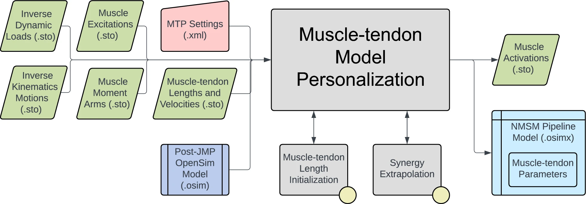
Data for IK joint motions, ID joint loads, and processed muscle excitations have already been provided. A post-JMP OpenSim model has also been provided. Muscle moment arms, and muscle-tendon lengths and velocities will be calculated in the first task for this module. In the next task, data will be processed to be in the correct format to use the MTP tool and the remainder of the NMSM Pipeline. Finally, you will conclude this module by running MTP.

Task 1: Muscle Analysis

A key step towards using MTP is to calculate muscular kinematic quantities such as moment arms, and muscle-tendon lengths. These quantities can be calculated using OpenSim’s Muscle Analysis (MA) tool. The MA tool is a subtool of OpenSim’s Analysis tool. A short guide to the Analysis tool can be found here.

The MA tool uses joint motions to calculate muscle-tendon lengths and muscle-moment arms about every joint using geometry calculations. Every modeled muscle has two attachment points on separate bodies such that they cross one or more joints and can apply moments about those joints. Anatomical muscles also have complex interactions with the bodies they’re attached to. The OpenSim model used in this tutorial represents these interactions using wrapping surfaces that define how muscles wrap around bones. These wrapping surfaces can be visualized in the OpenSim GUI by expanding the bodies tab under the model and then expanding individual bodies. The MA tool provides a quick and easy way to perform geometry calculations with these wrapping surfaces.

Step 1: Muscle analysis for gait

In this step, you will conduct MA on gait motion to calculate moment arms and muscle-tendon lengths throughout the gait cycle. These quantities will then be used in the main body of MTP to calculate muscle forces and corresponding joint moments. The input data files needed for this task step are in the inputData directory.

Load the model UF_Subject_4_Scaled_JMP.osim into the OpenSim GUI
Open the Analyze tool
Load the motion file Trial10_IKResults.mot
Change the prefix to Trial10 a. This changes the prefix added at the beginning of every file created by MA. This is important for file organization
Change the output directory to MuscleAnalysis\MAData
Under the Analyses tab, add a MuscleAnalysis task.
Edit the MuscleAnalysis task and ensure that the tool will compute moment arms for all muscles and all lower body coordinates.
Run the Muscle Analysis tool.
Verify that the tool creates files inside MuscleAnalysis\MAData that all have the prefix Trial10.
Bug Note
There is a bug with MA in which the gastrocnemius muscles have moment arms about the hip. To work around this, copy and paste the MA files inside input data to your new MA folder. These files should replace some of the files you just calculated.

Step 2: Muscle analysis for passive moment data

The next MA run will be done on passive joint moment data. MTP uses passive moment data inside Muscle-tendon Length Initialization (MTLI) to generate a good initial guess for the main MTP optimization.

MTLI uses published passive joint moment data. As described earlier, joints are moved through their full range of motion with other joints fixed at constant values. Joint moments are then measured using a dynamometer as the joint moves through its range of motion. These data are described below:

Thelen_AnklePassive_01 – Ankle passive moments with the fixed at knee at 0°
Thelen_AnklePassive_02 – Ankle passive moments with the fixed at knee at 15°
Thelen_AnklePassive_03 – Ankle passive moments with the fixed at knee at 60°
Thelen_AnklePassive_04 – Ankle passive moments with the fixed at knee at 110°
Thelen_HipPassive_01 – Hip passive moments with the knee fixed at 15°
Thelen_HipPassive_02 – Hip passive moments with the knee fixed at 60°
Thelen_HipPassive_03 – Hip passive moments with the knee fixed at 90°
Thelen_HipPassive_04 – Hip passive moments with the knee fixed at 110°
Thelen_KneePassive_01 – Knee passive moments with the ankle fixed at 20°
Thelen_KneePassive_02 – Knee passive moments with the ankle fixed at -15°
Thelen_KneePassive_03 – Knee passive moments with the hip fixed at 45°
Thelen_KneePassive_04 – Knee passive moments with the ankle fixed at 20° and the hip fixed at -15°

Inside the MuscleAnalysis folder, there are two folders thelen_r and thelen_l that contain passive joint moment data for then right and left legs respectively. They contain folders IKData and IDData, where IDData contains the passive joint moments, and IKData contains the corresponding joint angles. You will run MA for all 12 motion trials in IKData, for both legs.

Open the Matlab file passiveTrialMuscleAnalysis.m
Edit the variable thelenFolder to say either thelen_r or thelen_l
Edit the variable modelFileName to be the full path to your .osim model file.
Run the Matlab script.
Repeat for the other leg.

These steps should create a folder called MAData inside each of thelen_r or thelen_l, and subfolders for each trial with muscle analysis files inside each folder. If these are not there, verify that all your file paths and names are correct.

Task 2: Data preprocessing

The next step in this module will be to process your data to get it into the correct format for the remainder of the NMSM Pipeline. This process will contain several parts, all of which are contained in the NMSM Pipeline’s preprocessing tool:

Process EMG data: Starting from the raw EMG file, the script high pass filters, demeans, rectifies, and low pass filters the EMG signals. Next, any remaining negative EMG values are set to zero. EMG signals are then offset so that the minimum value of each signal is 0. Finally, EMG signals are normalized so that the max value of each signal is 1.
Create muscle-tendon velocities: The script low pass filters the muscle-tendon lengths created by Muscle Analysis, splines the filtered data using GCV splines, and then differentiates the filtered data.
Crop and resample data: A user input to preprocessing is a set of time pairs for which the data should be cropped to. One file is created for each time pair specified by the variable trialTimePairs. The data are then splined and resampled to have 101 time points per trial.
Lowpass filter data: All data are low pass filtered using the cutoff frequency specified by inputSettings.cutoffFrequency.

Data preprocessing is contained entirely in the script Preprocessing\preprocessing.m. The EMG data has already been processed, so those corresponding lines of code are commented out.

Open Preprocessing\preprocessing.m.
Edit lines 12-17 with the paths to your data files.
We want to crop the data to one gait cycle (right heelstrike to right heelstrike). You must find the start time and the end time of the right heel strikes. To do this, open the file Preprocessing\plotInputGroundReactions.m and find the time of the first and second right heel strike (rounded down to the nearest 0.01s. ie if there is force starting at 0.98 seconds, round down to 0.97s).
Edit startTime and endTime to be the times you found above.
info
These variables specify the time ranges we want to crop the data into. This time pair isolates one single gait cycle that we will use for the rest of our modeling.
Explore the preprocessed directory that was created in your Preprocessing folder. This folder contains 5 folders for EMG data, IK data, ID data, GRF data, and MA data. Keep note of where this folder is. You will be using it for the rest of the tutorial.
danger
Do not change the name of any folders or files inside preprocessed. This tool outputs data in a format that the NMSM Pipeline expects from here on out. Changing any of these file or folder names will result in errors.
Visualize your preprocessing results with the function plotPreprocessing.m
Verify that all data look good (ie minimal noise, no sharp discontinuities, other data quality issues)

Task 3: Muscle-tendon Personalization

Now that you have preprocessed data, you can move onto using the NMSM Pipeline’s Muscle-tendon Personalization (MTP) tool. This tool will make use of the preprocessed data you just created, so there is no more work to be done for input data.

MTP will track this processed experimental data to fit Hill-type muscle model parameters for our model such that the joint moments generated by muscle forces match ID joint moments. For this module, you will iterate through MTP solutions, changing cost term parameters until you arrive to a physiologically realistic solution.

Step 1: Explore muscle groups

Open the OpenSim model UF_Subject_4_Scaled_JMP.osim in the OpenSim GUI.
Under the Forces tab on the model, explore the muscles available.
Take note of the extra groups added.
info
These are added for organization so that MTP/NCP knows which model muscles to group together in the optimization.

The four important muscle groups are:

Activation Muscle Groups – Muscles that we would expect to have similar activation profiles (ie lateral hamstrings; BFSH and BFLH will have similar activations to each other). These groups all have ActivationGroup in their name.
Normalized Fiber Length Muscle Groups – Muscles that we would expect to have similar normalized fiber lengths. These groups all have NormalizedFiberLengthGroup in their name.
Collected EMG Muscle Groups – Muscle groups that we do have experimental EMG data for. Unlike the other groups, these must have the same name as the respective EMG channel name your EMG data file. They cannot be named [muscle]_collectedEmgMuscleGroup unless you change the corresponding names in your EMG data file Preprocessing\preprocessed\EMGData\gait_1.sto
Missing EMG Muscle Groups – Muscle groups that we do not have experimental EMG data for. These groups all have MissingEMGChannelGroup in their name. The activation muscle groups and normalized fiber length muscle groups are organized based on how muscles are grouped anatomically. For example, we assume that your vastus muscles (three muscles that are a part of your quadriceps) will all have similar normalized fiber lengths and activation profiles because they serve similar functions. The collected and missing EMG muscle groups vary based on the dataset you are using, and which muscles have EMG data available.

The muscle groups for this tutorial are premade for you but it is important to study them and understand why certain muscles are grouped together.

Step 2: Create your base settings

You will need to create different settings files for the right and left leg. The reason for separating the legs is because SynX does not support multiple synergy sets. For this project, we are using 2 synergy sets – right leg and left leg. Therefore, MTP will need to be split up between the left and right leg. We will start with the right leg.

Load your premade post-JMP model UF_Subject_4_Scaled_JMP.osim into the OpenSim GUI
Open the Muscle-tendon Personalization Tool GUI
Set the Input Osimx File to GroundContactPersonalization\gcpResults\UF_Subject_4_Scaled_JMP_gcp.osimx
Set the Input Data Directory to Preprocessing\preprocessed
Set the Output Results Directory to MuscleTendonPersonalization\MTPResultsRightV1
Set your coordinate list to (hip_flexion_r, hip_adduction_r, hip_rotation_r, knee_angle_r, ankle_angle_r, subtalar_angle_r)
Set your Activation Muscle Groups to all right leg activation groups
tip
You can use the Filter by box at the top of the selection window to search for only right leg activation groups
Set your Normalized Fiber Length Muscle Groups to all right leg fiber length groups
Set your Missing EMG Muscle Groups to all right leg missing EMG groups
Set your Collected EMG Muscle Groups to all right leg EMG channels (Look at Preprocessing\preprocessed\EMGData\gait_1.sto)
Enable Muscle Tendon Length Initialization
Set the Passive Data Input Directory to MuscleAnalysis\thelen_r
Enable Muscle Tendon Synergy Extrapolation with 6 synergies
Save this settings file.
Repeat the above steps for the left side of the body, changing all necessary fields.
note
You will need to change the Input Osimx File to be the file that is output from the right side MTP run. This file does not exist yet, so just copy and paste the following text into the field: MTPResultsRightV1\UF_Subject_4_Scaled_JMP_gcp_mtp.osimx
Open MuscleTendonPersonalization\runMTP.m, and edit the settings files name and run the script.
note
It’s important that you run the right leg first because we use the output osimx file from the right leg as the input osimx file for the left leg. MTP does not use any information from the input osimx file in the optimization. The purpose of the input osimx file is so that MTP can concatenate left leg results to the right leg osimx file, keeping everything in the same file.

Step 3: Iterate through MTP solutions

Now that your first MTP run is complete, the next step is to iterate through settings files to fine tune a solution. To fine tune an MTP solution, there are generally 4 parameters you should change:

Minimum and maximum allowable normalized fiber lengths – These terms dictate the range that we allow the normalized fiber length to fall in, and how heavily we punish normalized fiber lengths outside that range.
Experimental quantity tracking terms – These terms affect how closely the optimization tracks joint moments.
a. passive_joint_moment in MTLI: How closely passive joint moments should be tracked in MTLI
b. measured_inverse_dynamics_joint_moment in SynX: How closely all joint moments in the model should track experimental joint moments.
Reduce max allowable error to prioritize SynX muscles more.
c. inverse_dynamics_joint_moment in MTP: How closely joint moments produced by muscles with experimental EMG data should track experimental joint moments.
Reduce max allowable error to use experimentally measured muscles more.

Max allowable errors and error centers for muscle group-based cost terms – These terms punish deviations between muscles in a group.
a. grouped_normalized_muscle_fiber_length
b. grouped_emg_scale_factor
c. grouped_electromechanical_delay
Regularization terms – These terms punish deviations in muscle-tendon parameters away from the error center and ensure the solution is unique.
a. optimal_muscle_fiber_length
b. tendon_slack_length
c. passive_muscle_force
d. activation_time_constant
e. activation_nonlinearity_constant
f. emg_scale_factor
g. muscle_excitation_penalty

Some common problems in an MTP solution and corresponding solutions are:

Poor joint moment tracking quality (RMSE > 10Nm) → Decrease moment tracking max allowable error
Large muscle activations (Max activation > 0.7 during gait) → Decrease max allowable error/error center for emg_scale_factor or muscle_excitation_penalty.
Large passive muscle forces (Max passive force > 100) → Decrease max allowable error on maximum_normalized_muscle_fiber_length, or passive_muscle_force
Large difference between muscle activations and muscle excitations → Decrease max allowable error on activation_nonlinearity_constant, or activation_time_constant
Large difference in activations or normalized fiber lengths between muscles in a group → Decrease max allowable error on grouped_normalized_muscle_fiber_length, grouped_emg_scale_factor, or grouped_electromechanical_delay
Under/overuse of unmeasured muscles → Change max allowable error on extrapolated_muscle_activation and residual_muscle_activation

Iteration 1 The first problem we will address is the large passive forces, especially in the calf and quad muscles. We will address this problem in a few ways. First, we will punish normalized fiber lengths falling outside of the optimal range of 0.8-1.0. Next, we will choose to optimize absolute length changes for optimal fiber length and tendon slack length (units of meters) instead of scale factors.

Create copies of your settings files and rename them.
For your new settings files, remember to update your <results_directory> fields for both files, and your <input_osimx_file> field for the left settings file:
We will also first the minimum normalized fiber length to avoid the normalized fiber length dropping too low. This will push the muscle fiber lengths closer to the ideal working range of 0.6-1 Change the following xml elements inside <MuscleTendonLengthInitialization>:
```
<max_normalized_muscle_fiber_length>1</max_normalized_muscle_fiber_length>
<min_normalized_muscle_fiber_length>0.8</min_normalized_muscle_fiber_length>
```
note
These elements do not affect the equations themselves. The "ideal working range" of a muscle is still 0.6-1. These terms simply change the cost terms to push the fiber lengths into a different range.
Passive forces are caused by normalized fiber lengths exceeding a value of 1, so we can reduce the max allowable error on the maximum normalized fiber lengths inside MTLI to more harshly punish normalized fiber lengths above 1. Change the following cost terms inside <MuscleTendonLengthInitialization>:
```
<RCNLCostTerm>
    <is_enabled>true</is_enabled>
    <type>maximum_normalized_muscle_fiber_length</type>
    <max_allowable_error>0.01</max_allowable_error>
</RCNLCostTerm>
```
note
This cost term will now more harshly punish normalized fiber lengths exceeding the value in <max_normalized_muscle_fiber_length>. You can use the other cost term with type maximum_normalized_muscle_fiber_length to punish fiber lengths falling below the value in <min_normalized_muscle_fiber_length>
To avoid over restricting the optimization, we can reduce the moment tracking value for MTLI as well. Change the following cost terms inside <MuscleTendonLengthInitialization>:
```
<RCNLCostTerm>
    <is_enabled>true</is_enabled>
    <type>passive_joint_moment</type>
    <max_allowable_error>15</max_allowable_error>
</RCNLCostTerm>
```
Next, we can change the optimization to optimize length parameters using absolute lengths instead of relative lengths. The previous optimization changed the scale factors of the optimal fiber length and tendon slack length. We will change this to optimize absolute changes in length, instead of scale factors. Inside <MuscleTendonLengthInitialization>:
Copy and paste the following lines to tell MTLI to optimize absolute lengths instead of scale factors:
```
<optimize_absolute_length_changes>true</optimize_absolute_length_changes>
```
Change the following cost terms so that they work with absolute length changes as well:
```
<RCNLCostTerm>
    <is_enabled>true</is_enabled>
    <type>optimal_muscle_fiber_length</type>
    <max_allowable_error>0.005</max_allowable_error>
    <error_center>0</error_center>
</RCNLCostTerm>
```
```
<RCNLCostTerm>
    <is_enabled>true</is_enabled>
    <type>tendon_slack_length</type>
    <max_allowable_error>0.005</max_allowable_error>
    <error_center>0</error_center>
</RCNLCostTerm>
```
info
An error center of 0 for absolute length changes means that the cost term is trying to keep the optimal fiber length and tendon slack lengths the same as their initial values.

Finally, inside the main optimization, we can reduce the max allowable error on the passive force cost term. Change the following cost term:

<RCNLCostTerm>
    <is_enabled>true</is_enabled>
    <type>passive_muscle_force</type>
    <max_allowable_error>10</max_allowable_error>
</RCNLCostTerm>

After running iteration 1, all passive forces should be below 50N. All normalized fiber lengths should be mostly between the range of 0.6-1.0. Some normalized fiber lengths may be a little bit above 1, but there should be a noticeable improvement over the initial MTP run.

Iteration 2:

The next observation is that certain muscles’ activations are significantly different from their excitations, beyond a simple time shift (psoas & recfem for example). Also, some muscles have very large muscle activations which is not realistic during gait (Left leg psoas and iliacus). We will first address these problems by lowering the max allowable error on the activation non-linearity constant. This will punish high non-linearities that are causing muscle activations to have much higher amplitude than the corresponding muscle excitations. Next, we will tighten max allowable errors on muscle-excitations to punish the large muscle excitations.

Create copies of your settings files and rename them.
For your new settings files, remember to update your <results_directory> fields for both files, and your <input_osimx_file> field for the left settings file.
Change the following cost terms in both settings files:
```
<RCNLCostTerm>
    <is_enabled>true</is_enabled>
    <type>muscle_excitation_penalty</type>
    <max_allowable_error>0.3</max_allowable_error>
    <error_center>0.3</error_center>
</RCNLCostTerm>
```
note
This change will punish excitations from getting too high. Deviations away from 0.3 ± 0.3 will be punished, so excitations greater than 0.6 will be punished. This cost term can also be used to punish excitations from being too low if you wish to do so.
```
<RCNLCostTerm>
    <is_enabled>true</is_enabled>
    <type>emg_scale_factor</type>
    <max_allowable_error>0.3</max_allowable_error>
    <error_center>0.3</error_center>
</RCNLCostTerm>
```
note
This change will also punish excitations from getting too high, but works with EMG scale factors rather than excitation magnitude.
```
<RCNLCostTerm>
    <is_enabled>true</is_enabled>
    <type>activation_nonlinearity_constant</type>
    <max_allowable_error>0.005</max_allowable_error>
    <error_center>0</error_center>
</RCNLCostTerm>
```
note
Tightening this cost term will move muscle activations closer to their excitations to fix muscles like the psoas that have excessively different shapes of their activations and excitations

Iteration 3:

This last iteration will address issues with SynX activations. Specifically, the right side SynX muscles (sartorius, piriformis, and quadratus femoris) are overactivated on the right leg and underactivated on the left leg. We will change this by tightening the max allowable errors on SynX. This iteration will also use different max allowable errors for the left and right sides.

Question

Why might we use different max allowable errors for the left and right sides?

Create copies of your settings files and rename them.
For your new settings files, remember to update your <results_directory> fields for both files, and your <input_osimx_file> field for the left settings file.
Right side:
a. Inside <MTPSynergyExtrapolation>, change the following cost term:
```
<RCNLCostTerm>
    <is_enabled>true</is_enabled>
    <type>extrapolated_muscle_activation</type>
    <max_allowable_error>0.1</max_allowable_error>
</RCNLCostTerm>
```
note
This cost term punishes the overuse of SynX muscles that we see in the right leg.
b. Inside <MTPTask>, change the following cost terms:
```
<RCNLCostTerm>
    <is_enabled>true</is_enabled>
    <type>inverse_dynamics_joint_moment</type>
    <max_allowable_error>3</max_allowable_error>
</RCNLCostTerm>
```
note
This cost term is adjusted to account for the added restriction to SynX. You generally do not want to have all of your max allowable errors be too low or the optimizer will struggle to find the optimal solution. ::
Left side:
a. Inside <MTPSynergyExtrapolation>, change the following cost terms:
```
<RCNLCostTerm>
    <is_enabled>true</is_enabled>
    <type>measured_inverse_dynamics_joint_moment</type>
    <max_allowable_error>1</max_allowable_error>
</RCNLCostTerm>
```
```
<RCNLCostTerm>
    <is_enabled>true</is_enabled>
    <type>extrapolated_muscle_activation</type>
    <max_allowable_error>1</max_allowable_error>
</RCNLCostTerm>
```
note
These cost term changes are doing the opposite of what we did for the right leg. SynX muscles were being underused on the left leg and so we tighten moment tracking term and loosen the extrapolated muscle excitation term to incentivize SynX to do more.
b. Inside <MTPTask>, change the following cost term:
```
<RCNLCostTerm>
    <is_enabled>true</is_enabled>
    <type>inverse_dynamics_joint_moment</type>
    <max_allowable_error>1</max_allowable_error>
</RCNLCostTerm>
```
note
This cost term is changed to work in conjunction with the changes in SynX. By raising the max allowable error on the moment tracking for measured muscles, we are allowing SynX muscles to activate more.

Deliverables

Submit your final plots of joint moments, normalized fiber lengths, muscle activations, and muscle passive forces for both legs.
In 1-2 sentences, explain how the MTP optimization works.
In 2-3 sentences each, explain how MTLI and SynX work, and why MTP needs them.
Summarize each MTP iteration you did. Information to include is:
a. What was the goal of the iteration?
b. What muscles were you aiming to fix?
b. Did the iteration achieve its goal?
Briefly explain why the final settings files were different between the legs (Hint: what problem were we trying to solve in iteration 3? Was it the same problem for both legs?)
Compare the muscle activations between the left and right sides. Are there any muscles that have significantly different activations on the left and right sides?
Do you think that the final solution you got for MTP is good enough to move forwards? Why or why not?
If you were to do one more MTP iteration, what would your goal be? What muscles are you trying to fix, and what cost terms would you change to achieve this goal?
When selecting the joint moments to match during MTP, we didn’t use the knee adduction moment or the mtp (toes) moment. Why didn’t we use these moments?
a. Toes: (Hint: Do we have joint moments for the toes? Why or why not? If not, how could we solve for toes joint moments?)
b. Knee adduction: (Hint: What generates the knee adduction moment? Remember that the net moment about a joint is given by: $M^{net}=M^{contact}+M^{muscle}+M^{ligament}$ )
In one paragraph explain why MTP is important for muscle-driven predictive simulations.

MODULE 1: MUSCLE-TENDON PERSONALIZATION

Task 1: Muscle Analysis​

Step 1: Muscle analysis for gait​

Step 2: Muscle analysis for passive moment data​

Task 2: Data preprocessing​

Task 3: Muscle-tendon Personalization​

Step 1: Explore muscle groups​

Step 2: Create your base settings​

Step 3: Iterate through MTP solutions​

Deliverables​