MODULE 4: VERIFICATION AND DESIGN OPTIMIZATION
In this module, you will use the NMSM Pipeline Design Optimization (DO) tool to design one or two personalized clinical treatments that reduce the peak adduction moment in both knees of a subject with bilateral medial compartment knee osteoarthritis. One treatment optimization problem will involve the design of personalized high tibial osteotomy surgery while the other will involve the design of personalized gait modifications. Undergraduate students are required to complete only one of the two treatment optimization problems and may choose between the two, while graduate students are required to complete both treatment optimization problems.
For both treatment optimization problems, you will need to perform a Verification Optimization (VO) followed by a Design Optimization. Your Verification Optimization will start from your Tracking Optimization (TO) solution to confirm that the torque controls produced by your TO run generate the correct lower body walking motion and ground reactions without tracking those quantities in the cost function. Similarly, your subsequent Design Optimization will start from your Verification Optimization solution to predict how the modeled treatment will affect the subject’s walking function and knee adduction moment peaks.
The VO and DO runs for this module will be performed using the following model and data files:
• OpenSim model file: Full_Body_Walking_Model-Post_JMP.osim
• NMSM Pipeline model file: Full_Body_Walking_Model-Post_GCP.osimx
• Inverse kinematics, ground reaction, and inverse dynamics data files: found in your TO results folder toResults.
The general Verification Optimization and Design Optimization processes to be performed for both treatment optimization problems are described in the two module tasks below. Following this general description, specific details are provided for how these general processes should be modified to account for the unique aspects of each treatment optimization problem.
Task 1: Verification Optimization
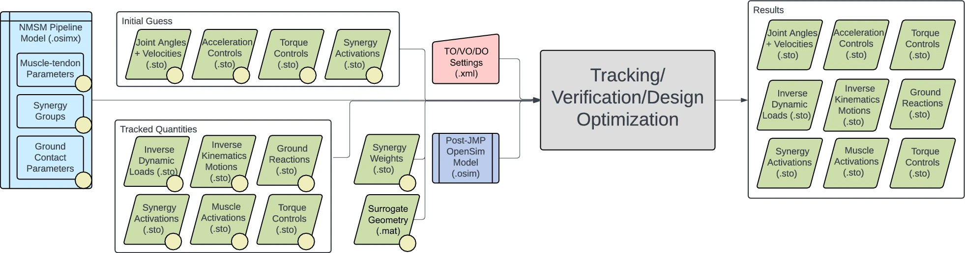
For this module task, you will used the NMSM Pipeline Verification Optimization tool to verify that the lower body joint torque controls found by your Tracking Optimization produce the same walking motion and ground reactions as did your Tracking Optimization but without tracking those quantities in the optimization cost function. This “sanity check” optimization will seek to minimize changes in your Tracking Optimization lower body torque controls and upper body joint motions so that a dynamically consistent near-periodic walking motion is produced. Results generated by your Tracking Optimization will provide the starting point for your Verification Optimization. The interaction between tool settings, data, and models required to perform this module task is shown in the figure below:
Your VO run will serve as a “dry run” for formulating the optimal control problem that you will solve in a subsequent DO run. You can think of your VO run as a DO run without the addition of the treatment design element. Normally a VO problem will be formulated primarily by removing cost and/or constraint terms from the original TO problem formulation. However, to make a VO run a “dry run” for a subsequent DO run, you will sometimes need to add one or more cost and/or constraint terms that were not present in your original TO problem formulation. When this situation arises, you will need to verify that the added cost and/or constraint terms do not affect the ability of your VO run to converge rapidly (i.e., within a few iterations) to your TO solution. If cost and/or constraint terms added to a VO problem formulation significantly increase the number of iterations required to converge, then the added cost and/or constraint terms are likely inconsistent with your base VO problem formulation containing only cost and constraint terms from your original TO run.
Step 1: Create your Verification Optimization settings file
- Copy your OpenSim model file
Full_Body_Walking_Model-Post_JMP.osimand your NMSM Pipeline model fileFull_Body_Walking_Model-Post_GCP.osimxto yourVOdata folder. - Create a VO settings file that is a modified version of your previous TO settings file.
- If you do not want to follow the process outlined below to create your VO settings file using the OpenSim GUI, you can instead copy your TO settings file to a new settings file named
VO_Settings.xml, openVO_Settings.xmlin a text editor, changeTrackingOptimizationTooltoVerificationOptimizationToolat the top and bottom of the file, and make any additional changes to the VO settings file as described below. - If you choose to use the OpenSim GUI to create your VO settings file, start by loading your post-JMP model
Full_Body_Walking_Model-Post_JMP.osiminto the OpenSim GUI. NMSM Pipeline tools will not be accessible in the OpenSim GUI Tools menu unless a model is loaded first. - Select Tools ⇨ User Plugins ⇨ rcnlPlugin.dll to load the NMSM Pipeline tools into the OpenSim GUI Tools menu.
- Select the Verification Optimization tool to set up a VO run that tracks the lower body torque controls and upper body joint motions from your TO run while making the simulated motion dynamically consistent.
- On the Settings tab, make the following choices in the Input section:
- Leave the pre-selected model name and path unchanged.
- For Osimx File:, choose
Full_Body_Walking_Model-Post_GCP.osimx. - For Initial Guess Dir:, choose your
toResultsdirectory. - For Tracked Quantities Dir:, also chose your
toResultsdirectory since the same data will be used for both an initial guess for the solution and the tracked data for the cost function and constraints. - For Trial Prefix:, input
Trial12_Gait.
- Still on the Settings tab, make the following choice in the Output section:
- For Results Dir:, create a new folder in your VO directory called
voResults.
- Still on the Settings tab, make the following choice in the Optimal Control Solver Settings File section:
- Click the folder icon on the Browse.. line and select the file
gpopsSettings.xmlin yourVOdirectory. This file contains default GPOPS-II optimal control solver settings that tend to work well for any Treatment Optimization problem.
- Still on the Settings tab, for the States Coordinates List:, select all moveable generalized coordinates in your OpenSim model
Full_Body_Walking_Model-Post_JMP.osim.
- On the RCNL Controllers tab, scroll down to the RCNL Torque Controller section, click on Edit…, and select the following coordinates to be controlled by torque controllers:
hip_flexion_r, hip_adduction_r, hip_rotation_r, knee_angle_r, ankle_angle_r, subtalar_angle_r, hip_flexion_l, hip_adduction_l, hip_rotation_l, knee_angle_l, ankle_angle_l, subtalar_angle_l.
Torque controllers are placed on only those joints that would be controlled by muscles if muscles were present in the model.
- On the Cost/Constraints tab, in the Cost Terms section at the top, click on Add… and add the cost terms and associated maximum allowable errors as outlined in the table below:
Type: controller_tracking (was `inverse_dynamics_load_tracking` in Tracking Optimization)
Components:
    hip_flexion_r_moment
    hip_adduction_r_moment
    hip_rotation_r_moment
    knee_angle_r_moment
    ankle_angle_r_moment
    subtalar_angle_r_moment
    hip_flexion_l_moment
    hip_adduction_l_moment
    hip_rotation_l_moment
    knee_angle_l_moment
    ankle_angle_l_moment
    subtalar_angle_l_moment
Max Allowable Error: 10
Type: generalized_coordinate_tracking
Components:
    mtp_angle_r
    mtp_angle_l
Max Allowable Error: 0.0873
Type: generalized_coordinate_tracking
Components:
    lumbar_extension
Max Allowable Error: 0.6981
Type: generalized_coordinate_tracking
Components:
    lumbar_bending
    lumbar_rotation
    arm_flex_r
    arm_add_r
    arm_rot_r
    elbow_flex_r
    arm_flex_l
    arm_add_l
    arm_rot_l
    elbow_flex_l
Max Allowable Error: 0.3491
These cost function terms come directly from your TO settings file except that every joint in the model is now controlled by either 1) controller tracking (lower body joints except for mtp joints), 2) generalized coordinate tracking (upper body joints plus mtp joints), or 3) no tracking (pelvis coordinates). In general, unlike for TO problem formulations, VO problem formulations generally have no joints controlled by both a cost function term and a constraint term (though this general rule can sometimes be violated to improve convergence for a subsequent DO run).
- Still on the Cost/Constraints tab, in the Constraint Terms section at the bottom, click on Add… and add the constraint terms outlined in the table below:
These constraint terms come directly from your TO settings file with no changes whatsoever.
Name: Kinetic consistency
Type: kinetic_consistency
Components:
    hip_flexion_r_moment
    hip_adduction_r_moment
    hip_rotation_r_moment
    knee_angle_r_moment
    ankle_angle_r_moment
    subtalar_angle_r_moment
    hip_flexion_l_moment
    hip_adduction_l_moment
    hip_rotation_l_moment
    knee_angle_l_moment
    ankle_angle_l_moment
    subtalar_angle_l_moment
Max/Min Error: 0.1/-0.1
Name: Residual force reduction
Type: root_segment_residual_load
Components:
    pelvis_tx_force
    pelvis_ty_force
    pelvis_tz_force
Max/Min Error: 1/-1
Name: Residual moment reduction
Type: root_segment_residual_load
Components:
    pelvis_tilt_moment
    pelvis_list_moment
    pelvis_rotation_moment
Max/Min Error: 0.1/-0.1
Name: Rotational coordinate periodicity
Type: generalized_coordinate_periodicity
Components:
    All rotational coordinates (not pelvis translation coordinates)
Max/Min Error: 0.0175/-0.0175
Name: Translational coordinate periodicity
Type: generalized_coordinate_periodicity
Components:
    pelvis_tx
    pelvis_ty
    pelvis_tz
Max/Min Error: 0.01/-0.01
Name: External force periodicity
Type: external_force_periodicity
Components:
    ground_force_2_vx
    ground_force_2_vy
    ground_force_2_vz
    ground_force_1_vx
    ground_force_1_vy
    ground_force_1_vz
Max/Min Error: 5/-5
Name: External moment periodicity
Type: external_moment_periodicity
Components:
    ground_moment_2_mx
    ground_moment_2_my
    ground_moment_2_mz
    ground_moment_1_mx
    ground_moment_1_my
    ground_moment_1_mz
Max/Min Error: 1/-1
Name: Rotational speed periodicity
Type: generalized_speed_periodicity
Components:
    All rotational coordinates (not pelvis translation coordinates)
Max/Min Error: 0.0873/-0.0873
Name: Translational speed periodicity
Type: generalized_speed_periodicity
Components:
    pelvis_tx
    pelvis_ty
    pelvis_tz
Max/Min Error: 0.1/-0.1
- Once you have finished configuring your VO settings file in the OpenSim GUI, Save your settings file in your VO folder and name it
VO_Settings.xml. Remember that if you want to read your VO settings file back into the OpenSim GUI to modify it (as opposed to simply modifying it in a text editor), you will need to use a different file name when you re-save the settings file due to a bug in the GUI implementation.
Step 2: Run your Verification Optimization settings file and plot your results
Once you have created your VO settings file, run the file and generate results by following the instructions below:
- Open Matlab, load the NMSM Pipeline project if necessary, and change directories to where your VO settings file is located.
- Run the VO tool in Matlab using the settings file you just saved by inputting the following commands into Matlab:
VerificationOptimizationTool('VO_Settings.xml')
Since none of the Treatment Optimization tools are parallelized through Matlab, you do not need to start a Matlab parallel pool to avoid having parallel processing startup impact your total wall clock time.
- If your VO problem is formulated well, your VO run should converge in just a few iterations. If your VO run requires more than 10 iterations to converge, then something is wrong with your VO problem formulation, and you should review your VO settings file to try to diagnose the source of the problem. A common problem is to have a constraint term that is redundant with or conflicts with a cost function term. For example, you could have a periodicity constraint on a quantity that you are tracking in the cost function, but the tracked quantity is less periodic than required by the periodicity constraint.
- Plot your VO results using Matlab function plotTreatmentOptimizationResultsFromSettingsFile.m as shown below:
plotTreatmentOptimizationResultsFromSettingsFile('VO_Settings.xml')
This function will output plots of your TO and VO generalized coordinates, generalized speeds, inverse dynamics loads, ground reaction forces and moments, and simulated torque controls. At the top of each subplot is a root-mean-square (RMS) error showing the difference between TO and VO quantities.
- For all plotted quantities, verify that your VO results are visually identical to your TO results with extremely low RMS errors.
Task 2: Design Optimization
Following generation of a successful Verification Optimization, you will use the NMSM Pipeline Design Optimization tool to design a personalized treatment that reduces the subject’s adduction moment peaks in both knees to a desired target value associated with an excellent long-term clinical outcome (Bryan et al., 1997). For either treatment optimization problem, results generated by your Verification Optimization will provide the starting point for your subsequent Design Optimization. The interaction between tool settings, data, and models required to perform this module task is shown in the figure below:
Step 1: Create your Design Optimization settings file
- Copy your OpenSim model file Full_Body_Walking_Model-Post_JMP.osim and your NMSM Pipeline model Full_Body_Walking_Model-Post_GCP.osimx file to your DO data folder.
- Create a DO settings file by modifying your VO settings file in a text editor
You could also create this settings file using the OpenSim GUI, but creating it in a text editor is the fastest and easiest approach).
- Copy your VO settings file to a new settings file named
DO_Settings.xml, openDO_Settings.xmlin a text editor, and make the following changes: • ChangeVerificationOptimizationTooltoDesignOptimizationToolat the top and bottom of the file. • Change the results directory todoResultsin your DO folder. • Change the initial guess and tracked quantities directories tovoResultswithin your VO folder.
Step 2: Run your Design Optimization settings file and plot your results
Once you have created your DO settings file, run the file and generate results by following the instructions below:
- Open Matlab, load the NMSM Pipeline project if necessary, and change directories to where your DO settings file is located.
- Run the DO tool in Matlab using the settings file you just saved by inputting the following commands into Matlab:
DesignOptimizationTool('DO_Settings.xml')
Since none of the Treatment Optimization tools are parallelized through Matlab, you do not need to start a Matlab parallel pool to avoid having parallel processing startup impact your total wall clock time.
3. If your DO problem is formulated well, your DO run should converge in less than 250 iterations.
4. Plot your DO results using Matlab function plotTreatmentOptimizationResultsFromSettingsFile.m as shown below:
plotTreatmentOptimizationResultsFromSettingsFile('DO_Settings.xml')
This function will output plots of your VO and DO generalized coordinates, generalized speeds, inverse dynamics loads, ground reaction forces and moments, and simulated torque controls. At the top of each subplot is an RMS error showing the difference between VO and DO quantities.
- Record the predicted absolute value of the peak knee adduction moment for both knees. Recall that your treatment design goal is to achieve a peak knee adduction of 2.5 %BW*Ht in both knees. For the subject being modeled (BW = 714 N, Ht = 1.70 m), this target value is equivalent to 30.3 Nm.
Step 3: Animate your predicted motion in OpenSim
- Load your OpenSim model
Full_Body_Walking_Model-Post_JMP.osiminto the OpenSim GUI twice. - For the first model, select File ⇨ Load Motion… and select the IK results file located in your
voResults\IKDatafolder. - For the second model, make the bones a different color, select File ⇨ Load Motion…, and select the IK results file located in your
doResults\IKDatafolder. - Sync the two motions and then animate them together at a slow Speed (e.g., 0.25). Note how much each knee in the predicted DO motion is medialized relative to the corresponding VO motion.
Given this general process for performing Verification Optimization and Design Optimization, problem-specific modifications required to solve each treatment optimization problem are described below:
Treatment Optimization Problem 1: Design of Personalized High Tibial Osteotomy Surgery
Step 1: Run a Verification Optimization
- Use the VO settings file described above with no modifications.
- Confirm that convergence to your TO solution occurs within just a few iterations.
Step 2: Add an HTO surgical correction to both tibias of your OpenSim model
Copy your OpenSim model
Full_Body_Walking_Model-Post_JMP.osimto a new model calledFull_Body_Walking_Model-Post_HTO.osim.Open
Full_Body_Walking_Model-Post_HTO.osimin a text editor and make the following changes:At the top of the file, change the model name to
Full_Body_Walking_Model-Post_HTO.Search for coordinate name
knee_adduction_rand change the default value to -0.0524 (3 deg), keeping the coordinate locked. This change sets the fixed knee adduction angle for the right tibia to 3 deg, emulating a 3 deg surgical correction in frontal plane leg alignment.Repeat for coordinate name
knee_adduction_l.Save the model with these changes.
Step 3: Run a Design Optimization using your post-HTO OpenSim model
- Use the DO settings file described above except with the input model file changed to your post-HTO OpenSim model.
- Confirm that your DO run converges within roughly 250 or fewer iterations.
Step 4: Repeat using surgical corrections of 6 deg and 9 deg for both tibias
- Run a Design Optimization using surgical corrections of 3 deg for both tibias.
- Repeat using surgical corrections of 6 deg for both tibias.
- Repeat using surgical corrections of 9 deg for both tibias.
- Record the predicted peak adduction moment for each knee in the deliverables table below.
Step 5: Perform a quadratic fit to estimate the optimal surgical correction for each tibia
Step 6: Perform a final Design Optimization using the optimal surgical corrections
Deliverables
- Wall clock time (min) and number of iterations for your final DO run.
Wall clock time: ____________ min
Number of iterations: ____________
- Peak adduction moment for both knees using surgical corrections of 3, 6, and 9 deg for both tibias (complete the table below):
| Peak Adduction Moment (Nm) | ||
|---|---|---|
| Surgical Correction (deg) | Right Knee | Left Knee |
| 3 | ||
| 6 | ||
| 9 | ||
- Optimal surgical correction for each tibia based on a quadratic fit to the data in the table above:
Optimal surgical correction for right tibia =   ____________ deg
Optimal surgical correction for left tibia =    ____________ deg
- Peak adduction moment for both knees predicted by your final DO run that used the post-HTO OpenSim model with optimal surgical correction for each tibia:
Predicted peak adduction moment for right knee =    ____________ Nm
Predicted peak adduction moment for left knee = ____________ Nm
Plots of your inverse dynamics loads from your final DO run as generated by Matlab plotting function
plotTreatmentOptimizationResultsFromSettingsFile.The DO settings file for your final DO run that used the post-HTO OpenSim model with optimal surgical correction for each tibia.
A brief paragraph discussing how well the quadratic fit worked for estimating the optimal amount of surgical correction needed for each tibia to achieve post-HTO surgery knee adduction moment peaks of 30.3 Nm for each knee.
Treatment Optimization Problem 2: Design of Personalized Gait Modifications
Step 1: Run a modified Verification Optimization
To match the optimization problem formulation used in (Fregly et al., 2007), make the following additions to the VO settings file described below:
- Add cost terms and associated maximum allowable errors as outlined in the table below:
Type: marker_position_tracking (x and z axes only)
Components:
    R_Heel
    R_Toe
    L_Heel
    L_Toe
Max Allowable Error: 0.0025
Type: body_orientation_tracking (x, y, and z axes using a yxz sequence)
Components:
calcn_r
calcn_l
torso
Max Allowable Error: 0.0175noteThese cost function terms make both feet follow the experimentally measured motion with respect to the lab coordinate system and make the torso follow the experimentally measured orientation with respect to the lab coordinate system. We do not track the foot marker y positions since we need to give the ground contact model freedom to equilibrate the model dynamics in the vertical direction.
- Add constraint terms and associated maximum/minimum errors as outlined in the table below:
Type: marker_position_deviation (x, y, and z axes)
Components:
    R_Heel
    R_Toe
    L_Heel
    L_Toe
Max/Min Error: 0.0025/-0.0025
Type: body_orientation_deviation (x, y, and z axes using a yxz sequence)
Components:
calcn_r
calcn_l
torso
Max/Min Error: 0.0175/-0.0175noteThese new constraint terms force the optimizer to find a solution where foot motion and torso orientation remain close to their experimental trajectories. Using a similar cost term and constraint term for marker positions and body orientations seems redundant but helps the optimizer converge more rapidly to a solution that matches the experimental foot motion and torso orientation closely.
This VO run should converge in roughly 10 or fewer iterations
Step 2: Run a Design Optimization using your post-JMP OpenSim model
Use the DO settings file described above (i.e., taken directly from your VO settings file) except with the addition of the following cost function term:
```
Type: inverse_dynamics_load_minimization
Components:
    knee_adduction_r_moment
    knee_adduction_l_moment
Max Allowable Error: 10
```RuntimeThis DO run should converge in roughly 250 or fewer iterations
Step 3: Repeat using max allowable errors of 15 and 20 Nm for both knee adduction moments
- Run a Design Optimization using maximum allowable errors of 10 Nm for both knee adduction moments.
- Repeat using maximum allowable errors of
15Nm for both knee adduction moments. - Repeat using maximum allowable errors of
20Nm for both knee adduction moments. - Record the predicted peak adduction moment for each knee in the deliverables table below.
Step 4: Perform a quadratic fit to estimate the optimal max allowable error for each knee
Step 5: Perform a final Design Optimization using the optimal max allowable error values
Deliverables
- Wall clock time (min) and number of iterations for your final DO run.
Wall clock time: ____________ min
Number of iterations: ____________
- Peak adduction moment for both knees using max allowable errors of 10, 15, and 20 Nm for both knee adduction moments (complete the table below):
| Peak Adduction Moment (Nm) | ||
|---|---|---|
| Max Allowable Error (Nm) | Right Knee | Left Knee |
| 10 | ||
| 15 | ||
| 20 | ||
- Optimal max allowable error for each knee adduction moment based on a quadratic fit to the data in the table above:
Optimal max allowable error for right knee adduction moment =   ____________ Nm
Optimal max allowable error for left knee adduction moment =    ____________ Nm
- Peak adduction moment for both knees predicted by your final DO run that used the optimal max allowable error for each knee adduction moment:
Predicted peak adduction moment for right knee =    ____________ Nm
Predicted peak adduction moment for left knee = ____________ Nm
- Plots of your inverse dynamics loads from your final DO run as generated by Matlab plotting function
plotTreatmentOptimizationResultsFromSettingsFile. - The DO settings file for your final DO run that used the optimal max allowable error for each knee adduction moment.
- A brief paragraph discussing how well the quadratic fit worked for estimating the optimal max allowable error for each knee adduction moment to achieve post-gait modification knee adduction moment peaks of 30.3 Nm for each knee.