MODULE 3: TRACKING OPTIMIZATION
In this module, you will use the NMSM Pipeline Tracking Optimization (TO) tool with your personalized skeletal model to create a dynamically consistent walking simulation that reproduces experimental joint motion, joint moment, and ground reaction data as closely as possible for a single gait cycle. Tracking Optimization results always provide the starting point for the NMSM Pipeline Treatment Optimization process. In the subsequent module, you will perform a Verification Optimization (VO) starting from your TO results to confirm that your TO results are reliable, followed by a Design Optimization (DO) starting from your VO results to design either a high tibial osteotomy surgery or a modified walking motion that reduces the peak adduction moment in both knees of a subject with bilateral medial knee osteoarthritis.
In preparation for this module, compare the root-mean-square translation, rotation, ground reaction force, and ground reaction moment errors produced using Coulomb and viscous friction in the two GCP runs you performed for the previous module. Select the NMSM Pipeline foot-ground contact model with the most physically realistic results and ideally the lowest errors. For “physically realistic,” look for ground reaction force and moment results that make sense physically (e.g., the ground reaction forces and moments should be zero during swing phase when the foot is off the ground and zero at the transitions into and out of contact). Copy this NMSM Pipeline model and give it the new name Full_Body_Walking_Model-Post_GCP.osimx.
The TO run for this module will be performed using the following model and data files:
• OpenSim model file: Full_Body_Walking_Model-Post_JMP.osim
• NMSM Pipeline model file: Full_Body_Walking_Model-Post_GCP.osimx
• Inverse kinematics data file: Trial12_Gait_IK_results_filtered.mot (to be cropped – this data file was an input to, not an output from, Ground Contact Model Personalization)
• Ground reaction data file: updated_Trial12_Gait_forces_filtered.mot (to be cropped)
• Inverse dynamics data file: Trial12_Gait_ID_results.sto (to be created and cropped)
Once all necessary input data files are available, they will be cropped to a single gait cycle between 2.235 to 3.280 seconds, which is the same gait cycle used for the Ground Contact Model Personalization process. The cropping process will be performed using Matlab program cropGaitData.m provided with the project.
Note that this step uses an updated rather than the original ground reaction data file. This updated file was produced by Ground Contact Model Personalization and contains a small shift in the electrical center location of each force plate. The electrical center is the point about which moments are summed for a force plate. The location of this point often contains small errors (especially for split-belt instrumented treadmills) that make the ground reaction data inconsistent with the video motion capture data. Ground Contact Model Personalization corrected for this inconsistency during the third GCP task that matched all three components of ground reaction moments as well as all three components of ground reaction forces.
Task 1: Inverse Dynamics
Step 1: Perform inverse dynamics using the gait trial experimental data.
Copy the ground reactions data file
updated_Trial12_Gait_forces_filtered.motfrom theGCP\gcpResults\GRFDatafolder for your selected friction model to your Inverse Dynamics folder and rename it Trial12_Gait_forces_filtered_updated.mot.Load model
Full_Body_Walking_Model-Post_JMP.osiminto the OpenSim GUI and select the Inverse Dynamics tool.On the Main Settings tab, make the following selections:
- Under Input, for the From … option, select your filtered inverse kinematics motion data file
Trial12_Gait_IK_results_filtered.mot, check the Filter coordinates checkbox, and enter 6 Hz. - Under Time, keep the default Time range to process as 0 to 4 seconds, which was populated when you selected your inverse kinematics motion file.
- Under Output, make the Directory your Inverse Dynamics data folder.
- Under Input, for the From … option, select your filtered inverse kinematics motion data file
On the External Loads tab, select the External Loads checkbox and click the pencil icon to bring up the External Forces set up window. In this window, select the ground reaction data to use as follows:
Click the folder icon next to Force data file and select your ground reactions data file
Trial12_Gait_forces_filtered_updated.mot.Click Add to add ground reaction data to the left and right feet. Use force plate 2 data for the right foot and force plate 1 data for the left foot. Make sure the force and torque are applied to the calcaneus body and that the force and point data are expressed in the ground coordinate system.
Save your ground reactions External Forces settings file (a sub-settings file within inverse dynamics) as
External_Forces_Settings_Gait.xmlusing he Save… button at the bottom of the External Forces window.
Once your Inverse Dynamics settings file is completed, save it to your hard disk using the Save… command at the bottom of the tool window and name it
ID_Settings_Gait.xml.Run your Inverse Dynamics analysis and verify that the default inverse dynamics results file
invese_dynamics.stowas saved to your Inverse Dynamics data folder. Rename this fileTrial12_Gait_ID_results.sto.The inverse dynamics results generated in this step cover more than the gait cycle of interest, since the spline fitting process used to calculate joint velocities and accelerations has end effects that distort the values of the derivatives near the start time and end time. Performing inverse dynamics over a larger time window than needed and then cropping the results to the desired time window afterward eliminates these end effects.
Step 2: Crop all of your input data files to one gait cycle
Open Matlab and change directories to your
Inverse Dynamicsdata folder.Run the provided Matlab program
cropGaitData.mwith no inputs. The program will automatically pick the correct gait trial data and crop it using a start time of 2.235 second and an end time of 3.280 seconds.After the program finishes, verify that new data files with the following names are present in your Inverse Dynamics data folder:
Trial12_Gait_IK_results_filtered_cropped.stoTrial12_Gait_ID_results_cropped.stoTrial12_Gait_forces_filtered_updated_cropped.sto
All three data files now have a .sto extension. OpenSim is agnostic between .mot and .sto file extensions but prefers the .sto extension. Consequently, from here forward, .sto files will be used throughout the Treatment Optimization process.
Task 2: Tracking Optimization
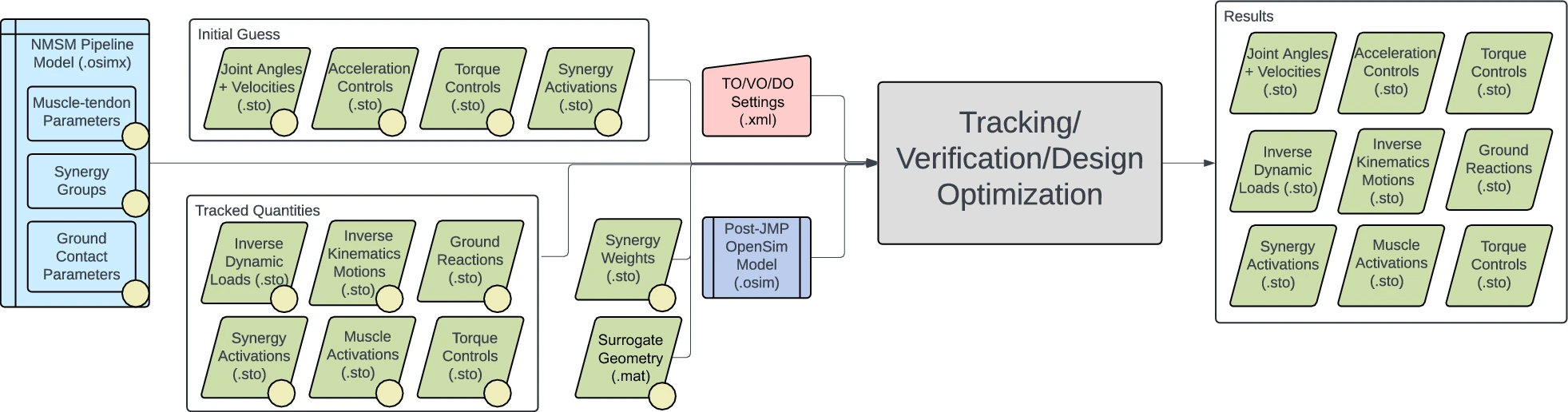
For this module task, you will used the NMSM Pipeline Tracking Optimization tool to produce a one-cycle dynamically consistent walking simulation based on your personalized post-JMP OpenSim model and your associated personalized post-GCP NMSM Pipeline foot-ground contact model. The optimization will seek to spread out errors in matching experimental joint motion from inverse kinematics, ground reaction forces and moments, and joint moments from inverse dynamics while driving the residual forces and torques acting on the pelvis segment to near zero. The personalized OpenSim/NMSM Pipeline skeletal model created by the Model Personalization process will provide the starting point for this module. The interaction between tool settings, data, and models required to perform this module task is shown in the figure below:
Step 1: Organize your input model and data files in preparation for your TO run
Copy your OpenSim model file
Full_Body_Walking_Model-Post_JMP.osimand your NMSM Pipeline modelFull_Body_Walking_Model-Post_GCP.osimxfile to your TO data folder.Create a folder called
inputDatawithin your TO data folder.Copy the three cropped gait data files created from your
Inverse Dynamicsfolder to yourinputDatafolder.Make the following changes within your
inputDatafolder:Move
Trial12_Gait_IK_results_filtered_cropped.stoto theIKDatafolder and rename itTrial12_Gait.sto.Move
Trial12_Gait_ID_results_filtered_cropped.stoto theIDDatafolder and rename itTrial12_Gait.sto.Move
Trial12_Gait_force_filtered_updated_cropped.stoto theGRFDatafolder and rename itTrial12_Gait.sto.
All three of these gait data files have the same file name by design. The folder in which each file is located tells the NMSM Pipeline what each data file is.
Step 2: Create your Tracking Optimization settings file
- Load the post-JMP model Full_Body_Walking_Model-Post_JMP.osim into the OpenSim GUI. NMSM Pipeline tools will not be accessible in the OpenSim GUI Tools menu unless a model to simulate is loaded first.
- Select Tools User Plugins rcnlPlugin.dll to load the NMSM Pipeline tools into the OpenSim GUI Tools menu.
- Select the Tracking Optimization tool to set up a TO run that reproduces the inverse kinematics, inverse dynamics, and ground reaction data for the one-cycle gait motion as closely as possible while making the simulated motion dynamically consistent.
- On the Settings tab, make the following choices in the Input section:
- Leave the pre-selected model name and path unchanged.
- For Osimx File:, choose
Full_Body_Walking_Model-Post_GCP.osimx. - For Initial Guess Dir:, choose your
inputDatadirectory. - For Tracked Quantities Dir:, also chose your
inputDatadirectory since the same data will be used for both an initial guess for the solution and the tracked data for the cost function and constraints. - For Trial Prefix:, input
Trial12_Gait.
- Still on the Settings tab, make the following choice in the Output section:
- For Results Dir:, create a new folder in your TO directory called
toResults.
- For Results Dir:, create a new folder in your TO directory called
- Still on the Settings tab, make the following choice in the Optimal Control Solver Settings File section:
- Click the folder icon on the Browse.. line and select the file
gpopsSettings.xmlin your TO directory. This file contains default GPOPS-II optimal control solver settings that tend to work well for any Treatment Optimization problem.
- Click the folder icon on the Browse.. line and select the file
- Still on the Settings tab, for the States Coordinates List:, select all unlocked (i.e., changeable) generalized coordinates in your OpenSim model
Full_Body_Walking_Model-Post_JMP.osim. DO NOT select any locked coordinates for your states. - On the RCNL Controllers tab, scroll down to the RCNL Torque Controller section, click on Edit…, and select the following coordinates to be controlled by torque controllers:
hip_flexion_r, hip_adduction_r, hip_rotation_r, knee_angle_r, ankle_angle_r, subtalar_angle_r, hip_flexion_l, hip_adduction_l, hip_rotation_l, knee_angle_l, ankle_angle_l, subtalar_angle_l.
Torque controllers are placed on only those joints that would be controlled by muscles if muscles were present in the model.
- On the Cost/Constraints tab, in the Cost Terms section at the top, click on Add… and add the cost terms and associated maximum allowable errors as outlined below:
Type: generalized_coordinate_tracking
Components:
    pelvis_tx
    pelvis_tz
Max Allowable Error: 0.02
Type: generalized_coordinate_tracking
Components:
    pelvis_tilt
    pelvis_list
    pelvis_rotation
    hip_flexion_r
    hip_adduction_r
    hip_rotation_r
    knee_angle_r
    ankle_angle_r
    hip_flexion_l
    hip_adduction_l
    hip_rotation_l
    knee_angle_l
    ankle_angle_l
Max Allowable Error: 0.1745
Type: generalized_coordinate_tracking
Components:
    subtalar_angle_r
    mtp_angle_r
    subtalar_angle_l
    mtp_angle_l
Max Allowable Error: 0.0873
Type: generalized_coordinate_tracking
Components:
    lumbar_extension
Max Allowable Error: 0.6981
Type: generalized_coordinate_tracking
Components:
    lumbar bending
    lumbar_rotation
    arm_flex_r
    arm_add_r
    arm_rot_r
    elbow_flex_r
    arm_flex_l
    arm_add_l
    arm_rot_l
    elbow_flex_l
Max Allowable Error: 0.3491
Type: generalized_speed_tracking
Components:
    pelvis_tx
    pelvis_tz
Max Allowable Error: 0.2
Type: generalized_speed_tracking
Components:
    pelvis_tilt
    pelvis_list
    pelvis_rotation
    hip_flexion_r
    hip_adduction_r
    hip_rotation_r
    knee_angle_r
    ankle_angle_r
    hip_flexion_l
    hip_adduction_l
    hip_rotation_l
    knee_angle_l
    ankle_angle_l
Max Allowable Error: 1.7453
Type: generalized_speed_tracking
Components:
    subtalar_angle_r
    mtp_angle_r
    subtalar_angle_l
    mtp_angle_l
Max Allowable Error: 0.8727
Type: generalized_speed_tracking
Components:
    lumbar_extension
    lumbar_bending
    lumbar_rotation
    arm_flex_r
    arm_add_r
    arm_rot_r
    elbow_flex_r
    arm_flex_l
    arm_add_l
    arm_rot_l
    elbow_flex_l
Max Allowable Error: 3.4907
Type: inverse_dynamics_load_tracking
Components:
    hip_flexion_r_moment
    hip_adduction_r_moment
    hip_rotation_r_moment
    knee_angle_r_moment
    ankle_angle_r_moment
    subtalar_angle_r_moment
    hip_flexion_l_moment
    hip_adduction_l_moment
    hip_rotation_l_moment
    knee_angle_l_moment
    ankle_angle_l_moment
    subtalar_angle_l_moment
Max Allowable Error: 10
Type: external_force_tracking
Components:
    ground_force_2_vx
    ground_force_2_vy
    ground_force_2_vz
    ground_force_1_vx
    ground_force_1_vy
    ground_force_1_vz
Max Allowable Error: 40
Type: external_moment_tracking
Components:
    ground_moment_2_mx
    ground_moment_2_my
    ground_moment_2_mz
    ground_moment_1_mx
    ground_moment_1_my
    ground_moment_1_mz
Max Allowable Error: 10
The pelvis_tx and pelvis_tz coordinates should be tracked lightly, since you need only a small amount of error for them to keep the pelvis over a unique location on the treadmill. You should never track the pelvis_ty coordinate since the pelvis height needs to adjust to allow the foot-ground contact models to equilibrate properly. All maximum allowable errors above were scaled up by a factor of two from their original values to speed up convergence. Maximum allowable errors for generalized coordinate tracking were selected so that lower body joint angles are tracked well to facilitate reproducing the correct inverse dynamics joint moments, ankle, subtalar, and toes angles are tracked very well to facilitate reproducing the correct ground reaction forces and moments, and upper body joint angles are tracked less well to balance out the dynamics. Maximum allowable errors for generalized speed tracking were generally chosen to be 10x greater than corresponding errors for generalized coordinate tracking. Inverse dynamic load tracking is applied to all joints for which an RCNL Torque Controller is present.
- Still on the Cost/Constraints tab, in the Constraint Terms section at the bottom, click on Add… and add the constraint terms outlined in the table below:
Name: Kinetic consistency
Type: kinetic_consistency
Components:
    hip_flexion_r_moment
    hip_adduction_r_moment
    hip_rotation_r_moment
    knee_angle_r_moment
    ankle_angle_r_moment
    subtalar_angle_r_moment
    hip_flexion_l_moment
    hip_adduction_l_moment
    hip_rotation_l_moment
    knee_angle_l_moment
    ankle_angle_l_moment
    subtalar_angle_l_moment
Max/Min Error: 0.1/-0.1
Name: Residual force reduction
Type: root_segment_residual_load
Components:
    pelvis_tx_force
    pelvis_ty_force
    pelvis_tz_force
Max/Min Error: 1/-1
Name: Residual moment reduction
Type: root_segment_residual_load
Components:
    pelvis_tilt_moment
    pelvis_list_moment
    pelvis_rotation_moment
Max/Min Error: 0.1/-0.1
Name: Rotational coordinate periodicity
Type: generalized_coordinate_periodicity
Components:
    All rotational coordinates (not pelvis translation coordinates)
Max/Min Error: 0.0175/-0.0175
Name: Translational coordinate periodicity
Type: generalized_coordinate_periodicity
Components:
    pelvis_tx
    pelvis_ty
    pelvis_tz
Max/Min Error: 0.01/-0.01
Name: External force periodicity
Type: external_force_periodicity
Components:
    ground_force_2_vx
    ground_force_2_vy
    ground_force_2_vz
    ground_force_1_vx
    ground_force_1_vy
    ground_force_1_vz
Max/Min Error: 5/-5
Name: External moment periodicity
Type: external_moment_periodicity
Components:
    ground_moment_2_mx
    ground_moment_2_my
    ground_moment_2_mz
    ground_moment_1_mx
    ground_moment_1_my
    ground_moment_1_mz
Max/Min Error: 1/-1
Name: Rotational speed periodicity
Type: generalized_speed_periodicity
Components:
    All rotational coordinates (not pelvis translation coordinates)
Max/Min Error: 0.0873/-0.0873
Name: Translational speed periodicity
Type: generalized_speed_periodicity
Components:
    pelvis_tx
    pelvis_ty
    pelvis_tz
Max/Min Error: 0.1/-0.1
For this problem, <min_error> should always be chosen to be the negative of <max_error>, though it need not be. Adding periodicity to the constraints makes the simulated gait cycle near-periodic, which is a required condition for performing predictive simulations of a single walking cycle in subsequent Design Optimization runs. The closer the specified constraints are to perfectly periodic, the longer the TO run will take to converge. A kinetic consistency constraint is required for all joints with an RCNL Torque Controller.
- Once you have finished configuring your TO settings file in the OpenSim GUI, Save your settings file in your
TOfolder and name itTO_Settings.xml. Remember that if you want to read your TO settings file back into the OpenSim GUI to modify it (as opposed to simply modifying it in a text editor), you will need to use a different file name when you re-save the settings file due to a bug in the GUI implementation.
Step 3: Run your Tracking Optimization settings file and plot your results
Once you have created your TO settings file, run the file and generate results by following the instructions below:
- Open Matlab, load the NMSM Pipeline project if necessary, and change directories to where your TO settings file is located.
- Run the TO tool in Matlab using the settings file you just saved by inputting the following commands into Matlab:
TrackingOptimizationTool('TO_Settings.xml')
Since none of the Treatment Optimization tools are parallelized through Matlab, you do not need to start a Matlab parallel pool to avoid having parallel processing startup impact your total wall clock time.
2 Plot your TO results using Matlab function plotTreatmentOptimizationResultsFromSettingsFile.m as shown below:
plotTreatmentOptimizationResultsFromSettingsFile('TO_Settings.xml')
This function will output plots of experimental and simulated generalized coordinates, generalized speeds, inverse dynamics loads, and ground reaction forces and moments, along with plots of simulated torque controls. At the top of each subplot is a root-mean-square error showing the difference between the experimental and simulated quantity.
The relative weighting of the cost function and constraint terms significantly affects the speed of Tracking Optimization convergence. Explore changing your TO settings file in the ways shown below and note how it changes both the solution and the number of iterations required for convergence:
• Multiply the <max_allowable_error> by 2 for each of your cost function terms.
• Divide the <max_allowable_error> by 2 for each of your cost function terms.
• Multiply the <max_error> and <min_error> by 2 for each of your constraint terms.
• Divide the <max_error> and <min_error> by 2 for each of your constraint terms.
Deliverables
- Wall clock time (min) and number of iterations for your TO run.
Wall clock time: ____________ min
Number of iterations: ____________
- RMS errors for both feet in matching experimental generalized coordinates (m or deg), generalized speeds (m/s or rad/sec), inverse dynamics loads (Nm), ground reaction forces (N), and ground reaction moments (Nm) (complete the table below):
| Generalized Coordinate (m or deg) | Generalized Speed (m/s or rad/s) | Inverse Dynamics Moment (NM) | |
|---|---|---|---|
| pelvis_tx_force | |||
| pelvis_ty_force | |||
| pelvis_tz_force | |||
| pelvis_tilt | |||
| pelvis_list | |||
| pelvis_rotation | |||
| pelvis_tx_force | |||
| pelvis_rotation | |||
| hip_flexion_r | |||
| hip_adduction_r | |||
| hip_rotation_r | |||
| knee_angle_r | |||
| ankle_angle_r | |||
| subtalar_angle_r | |||
| mtp_angle_r | |||
| hip_flexion_l | |||
| hip_adduction_l | |||
| hip_rotation_l | |||
| knee_angle_l | |||
| ankle_angle_l | |||
| subtalar_angle_l | |||
| mtp_angle_l | |||
| lumbar_extension | |||
| lumbar_bending | |||
| lumbar_rotation | |||
| arm_flex_r | |||
| arm_add_r | |||
| arm_rot_r | |||
| elbow_flex_r | |||
| arm_flex_l | |||
| arm_add_l | |||
| arm_rot_l | |||
| elbow_flex_l |
- RMS errors for both feet in matching experimental ground reaction forces (N) and ground reaction moments (Nm) (complete the table below):
| Ground Reaction (N or Nm) | |
|---|---|
| ground_force_2_vx | |
| ground_force_2_vy | |
| ground_force_2_vz | |
| ground_force_1_vx | |
| ground_force_1_vy | |
| ground_force_1_vz | |
| ground_moment_2_mx | |
| ground_moment_2_my | |
| ground_moment_2_mz | |
| ground_moment_1_mx | |
| ground_moment_1_my | |
| ground_moment_1_mz |
- Absolute values of the peak adduction moment for both knees in units of Nm and and in units of percent bodyweight x height (subject bodyweight was 714 N and height was 1.70 m).
| Units of Nm | Units of %BWxHT | |
|---|---|---|
| knee_adduction_r_moment | ||
| knee_adduction_l_moment |
- Plots of your generalized coordinate, generalized speed, inverse dynamics load, and ground reaction force and moments errors, as generated by Matlab plotting function
plotTreatmentOptimizationResultsFromSettingsFile. - Your TO settings file for the TO run whose results are shown in the tables above.
- A brief paragraph discussing what you believe to be the “largest” error in your TO results (realizing that different types of errors have different units), why you believe this error is the “largest one,” and one idea that could potentially improve it.