MODULE 2: GROUND CONTACT MODEL PERSONALIZTION

In this module, you will use the OpenSim Inverse Kinematics tool and the NMSM Pipeline Ground Contact Model Personalization (GCP) tool to personalize foot-ground contact model properties in a new NMSM Pipeline model to be associated with your post-JMP OpenSim model. The personalization process will be performed using marker motion and ground reaction data obtained from the gait trial.

Task 1: Inverse Kinematics for Gait Motion

The starting point for Ground Contact Model Personalization is always a post-JMP OpenSim model whose joint positions/orientations in the body segments, body scale factors, and/or marker locations on the body segments have been calibrated using the Joint Model Personalization tool. As indicated above, you will use model Full_Body_Walking_Model-Post_JMP.osim as your starting point. You will then perform an OpenSim Inverse Kinematics analysis on this model using one cycle of gait trial marker data to generate the input joint motions needed for performing Ground Contact Model Personalization. The interaction between tool settings, data, and models required to perform this module task is shown in the figure below:

The only experimental data needed for the Inverse Kinematics analysis is marker data contained in the gait trial datafile Trial12_Gait_markers.trc. This file contains data for all experimental markers, including those on the torso and arms.

Step 1: Perform inverse kinematics using the gait trial marker data.

1. Load model Full_Body_Walking_Model-Post_JMP.osim into the OpenSim GUI and select the Inverse Kinematics tool.

2. Under IK Trial, select the marker data from gait trial Trial12_Gait_markers.trc and keep the default time range from 0 to 4 seconds.

3. On the Weights tab, select following marker selections and use the following weights:

   Deselect:

   All medial and lateral toe, ankle, and knee markers.
   The non-central sacral markers
   Both shoulder markers and the back marker.

   Select:

   All remaining foot and pelvis markers using a weight of 10
   All tibia, arm, and chest markers using a weight of 1
   All thigh markers using a weight of 0.1
   The lumbar_rotation coordinate, set a Manual value of zero, and set the weight to 0.1

4. Name your Output Motion File Trial12_Gait_IK_results.mot.

5. Once your Inverse Kinematics settings file is completed, save it to your hard disk using the Save command at the bottom of the tool menu and name it IK_Settings_Gait.xml.

6. Run your Inverse Kinematics analysis and verify that your results file was written to your hard disk. If not, right click on IK Results in the GUI Navigator pane and select Save As to save the motion file to your hard disk.

7. The inverse kinematics results generated in this step cover more than the gait cycle of interest, since the filtering process to be performed in the next step introduces end effects. These effects distort each filtered curve near the start time and end time, causing significant errors in not only the filtered joint position data but also the joint velocity data to be calculated from it. Taking filtered inverse kinematics data from a time window that is not close to the start time or end time eliminates the presence of end effects caused by the filtering process.

Step 2: Filter your inverse kinematics motion file

1. Open Matlab and change directories to your Inverse Kinematics data folder.
2. Run the provided Matlab program filterIKResults.m without providing any inputs. The correct default inputs will be used automatically.
3. After the program finishes, verify that a new inverse kinematics motion file called Trial12_Gait_IK_results_filtered.mot is now present in your Inverse Kinematics data folder, and copy this file to your GCP data folder.
4. Filtered inverse kinematics results are needed since each GCP run will need to differentiate the IK joint position results to generate joint velocity results. These joint velocity estimates are in turn needed to calculate point velocities relative to ground for the contact elements placed on the bottom of each foot by the Ground Contact Model Personalization process. Contact element velocities are inputs to vertical contact force nonlinear damping and horizontal contact force friction calculations.
5. After generating your filtered inverse kinematics results file, open two versions of model Full_Body_Walking_Model-Post_JMP.osimin the OpenSim GUI, load the unfiltered motion into the first model, and load the filtered motion into the second model (it can help to make the second a model a different color). Then sync both motions and animate them together to ensure that the motion of the feet produced by the filtered IK results closely follow the motion of the feet produced by the unfiltered IK results.

Task 2: Ground Contact Model Personalization

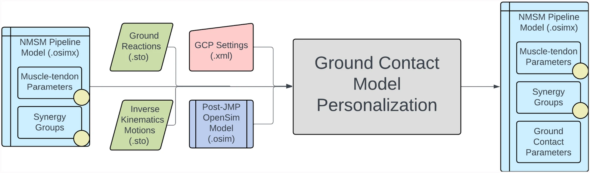
Now that you have inverse kinematics data available for your walking trial, you are ready to personalize the ground contact model properties of both feet in your model using the NMSM Pipeline’s Ground Contact Model Personalization tool. You will also need to use filtered experimental ground reaction data for this task. The interaction between tool settings, data, and models required to perform this module task is shown in the figure below:

The experimental data needed for the Ground Contact Model Personalization process is filtered inverse kinematic joint motion data and filtered ground reaction data contained in the datafiles located in the GCP folder and listed below:

• Trial12_Gait_IK_results_filtered.mot – filtered joint motion data for multiple walking cycles.
• Trial12_Gait_forces_filtered.mot – filtered ground reaction data for multiple walking cycles. Note that the sampling frequency for the ground reaction data has been decreased to match the sampling frequency of the marker and inverse kinematics data, which is a requirement for running the GCP tool.

Each datafile contains data for 4 seconds of walking. You will use only a single cycle of walking data, defined by a specified start time and end time, to personalize foot-ground contact models for both feet. Furthermore, the foot-ground contact model personalization process will be performed such that both feet possess the same contact model stiffness, damping, and friction properties.

Note that experimental marker data are not an input to this tool. Instead, your inverse kinematics results generated with tight tracking of foot markers are used as an input. Consequently, GCP tool runs actually track model (rather than experimental) marker trajectories generated by applying your filtered inverse kinematics motion to your OpenSim model.

For this module task, you will perform the Ground Contact Model Personalization process two times for both feet together by following a two-step process:

Step 1: You will personalize both feet together assuming Coulomb friction acts on each contact element.

Step 2: You will personalize both feet together assuming viscous friction acts on each contact element.

For both steps, you will create a GCP settings file using the Ground Contact Model Personalization tool in the OpenSim GUI. For each GCP settings file, you should use the following general guidelines:

1. Load the post-JMP model Full_Body_Walking_Model-Post_JMP.osim into the OpenSim GUI. NMSM Pipelilne tools will not be accessible in the OpenSim GUI Tools menu unless a model to personalize is loaded first.

2. Select Tools ⇨ User Plugins ⇨ rcnlPlugin.dll to load the NMSM Pipeline tools into the OpenSim GUI Tools menu.

3. Select the Ground Contact Model Personalization tool to set up a sequence of three GCP tasks to be saved as one GCP settings file that personalizes both feet together. Note that you will not create the three GCP tasks in the GUI. A sequence of three default tasks will be created for you automatically when you save your GCP settings file.

4. For the Input Model, choose your post-JMP model Full_Body_Walking_Model-Post_JMP.osim.

5. Leave Osimx File blank, since you will be creating a new .osimx file rather than appending to an existing one.

6. For Motion File, pick Trial12_Gait_IK_results_filtered.mot.

7. For Ground Reaction File, pick Trial12_Gait_forces_filtered.trc.

8. For Results Dir, create a folder called gcpResults within your GCP data folder and pick that folder.

9. Add two Ground Contact Personalization Surfaces, one for the right foot and one for the left foot. For both, use a Time Range of 2.235 to 3.280 seconds and a Belt Speed of 1.2 m/s. For Force Columns (_vx,y,z), Moment Columns (_mx,y,z), and Electrical Center (_px,y,z), use data from force plate 2 for the right foot and from force plate 1 for the left foot. For Hindfoot Body, pick the calcaneus calcn body for the appropriate foot. For various markers, pick the appropriate markers on each foot, noting that Medial Marker and Lateral Marker represent model markers placed on the toes axis of each foot. For the left foot, make sure to check the Left Foot checkbox.

10. The midfoot_superior model marker on each foot is a required input for this settings file since the point used for calculating ground reaction moments is the current location of the midfoot superior marker projected onto the floor. Ground reaction moments can be calculated about any desired point, and this choice of point keeps all three components of ground reaction moment “small” for the GCP calibration process. Choice of a point far from the center of the foot would produce large ground reaction moment components, and errors in those components would then swamp matching ground reaction force components during a GCP run.

11. Once you have completed these steps in the OpenSim GUI, Save your setting file in your GCP folder and name it GCP_Settings.xml. Note that your saved settings file will already have three pre-defined tasks included in it – a first task that focuses on reproducing just the vertical component of ground reaction force for both feet, a second that focuses on reproducing all three components of ground reaction force for both feet, and a third that focuses on reproducing all three components of ground reaction force and all three components of ground reaction moment for both feet. Each of these tasks contains default parameter values that will work well in most cases, and thus users do not have to create the three individual tasks themselves in the OpenSim GUI.

12. To finished configuring settings file GCP_Settings.xml that you created in the OpenSim GUI, open it in a text editor (ideally Notepad++ on Windows or BBEdit on Mac) and make the following changes to each <GCPTask>:

    • At the top of the settings file, change the value of <kinematics_filter_cutoff> to 6.

    • For the first task, change the value of <neighborStandardDeviation> to 0.3. For <RCNLCostTerm> items, change <max_allowable_error> for rotation to 0.0175, for ground_reaction_moment to 20, and for neighbor_spring_constant to 1000. Also add a new cost term called kinematic_periodicity and set its <max_allowable_error> to 3, which is a multiple of the ratio between corresponding original initial and final joint positions.

    • For the second task, make the same changes as for the first task plus change <max_allowable_error> for horizontal_grf to 5. Keep <restingSpringLength> set to the default selection of false.

    • For the third task, make the same changes as for the second task and leave <max_allowable_error> for ground_reaction_moment set to 0.5. In addition, set <electricalCenterX> and <electricalCenterZ> to true so that GCP will also calibrate the electrical center location of each force plate in the plane of the force plate.

    • At the bottom of the settings file, where settings are provided that apply to all tasks, change <initial_resting_spring_length> to 0.01, <initial_spring_constant> to 6000, <initial_damping_factor>to 0.5, and <initial_dynamic_friction_coefficient>to 0.3, <diff_min_change> to 1e-4, <step_tolerance> to 1e-5, and <max_iterations> to 25.

Bug Note

If you want to read a previously-created GCP settings file back into the OpenSim GUI to modify it, it will not work. Instead, you will need to modify existing GCP settings files directly using a text editor.

Once you have created and edited a GCP settings file, you will run the file and generate results by following the instructions below:

1. Open Matlab, load the NMSM Pipeline project if necessary, and change directories to where your GCP settings file is located.
2. Run the GCP tool in Matlab using the settings file you just saved by inputting the following commands into Matlab:

parpool
GroundContactPersonalizationTool('GCP_Settings.xml')

info

In this example, the name of the GCP settings file is GCP_Settings.xml. The parpool command will start a parallel pool of workers (which can take a minute or so) if your computer has multiple cores.

3. Plot your GCP results using the Matlab function plotGcpResultsFromSettingsFile.m as shown below:

plotGcpResultsFromSettingsFile('GCP_Settings.xml')

info

This function will output root-mean-square errors in matching ground reaction forces, ground reaction moments, hindfoot joint translations, hindfoot joint rotations, and toes joint rotations for your two personalized foot-ground contact models, along with a color plot showing the distribution of spring stiffness values over the bottom surface of the foot.

Before performing the two Ground Contact Model Personalization steps below, you should review the section describing the Ground Contact Model Personalization process in our recently published journal article describing the design and functionality of the NMSM Pipeline (Hammond et al., 2025). That section provides helpful information on how to formulate Ground Contact Model Personalization problems that reduce match ground reaction forces and moments closely without changing the motion of each foot substantially.

Step 1: Perform ground contact model personalization using Coulomb friction

1. Copy the GCP settings file created above and name it GCP_Settings_Coulomb.xml.
2. Open this file in a text editor.
3. Change the name of the <results_directory> to gcpResultsCoulomb.
4. Run Ground Contact Model Personalization with this settings file using the instructions provided above.

Step 2: Perform ground contact model personalization using viscous friction

1. Copy the original GCP settings file created above and name it GCP_Settings_Viscous.xml.
2. Open this file in a text editor.
3. Change the name of the <results_directory> to gcpResultsViscous.
4. Change <dynamicFrictionCoefficient> to false everywhere it appears in the file.
5. For the second and third tasks, change <viscousFrictionCoefficient> to true.
6. Change the value of <initial_dynamic_friction_coefficient> to 0.
7. Change the value of <initial_viscous_friction_coefficient> to 0.3.
8. Run Ground Contact Model Personalization with this settings file using the instructions provided above

Optional Exploration

For whichever friction model you decide is better, explore changing the following settings to see if they improve the ability of your personalized foot-ground contact models to reproduce the experimental ground reaction force/moment and foot motion data:

1. Run GCP without filtering the input inverse kinematics data (i.e., use the original inverse kinematics results file Trial12_Gait_IK_results.mot).

2. Double the grid density by changing the value of <grid_width> to 10 and <grid_height> to 22.

3. Reduce the value of <neighborStandardDeviation> to 0.2.

4. Reduce the <max_allowable_error> for neighbor_spring_constant to 500.

5. Reduce the <latching_velocity> to 0.05.

Deliverables

1. Wall clock time (sec) for your GCP runs with Coulomb friction and viscous friction:

   Coulomb friction wall clock time:   ____________ min
   
   Viscous friction wall clock time:   ____________ min

2. RMS errors for both feet in matching experimental ground reaction forces (N), ground reaction moments (Nm), toes and hindfoot rotations (deg), and hindfoot translations (m) when using Coulomb friction and viscous friction (complete the table below):

		Coulomb Friction		Viscous Friction
Quantity	Direction	Right Foot	Left Foot	Right Foot	Left Foot
RMS Force Error (N)	Anterior
	Vertical
	Lateral
RMS Moment Error (Nm)	X
	Y
	Z
RMS Rotation Error (deg)	Toes
	X
	Y
	Z
RMS Translation Error (m)	X
	Y
	Z

3. For each friction model and each foot, a plot comparing post-GCP ground reaction forces and moments with experimental ground reaction forces and moments.
4. For each friction model and one foot, a color plot showing the distribution of spring stiffness values over the bottom surface of the foot.
5. The GCP settings files for the two GCP runs whose results are shown in the table above.
6. Post-GCP NMSM Pipeline models Full_Body_Walking_Model-GCP_Coulomb.osimx produced by GCP using Coulomb friction and Full_Body_Walking_Model-GCP_Viscous.osimx produced by GCP using viscous friction.
7. A brief paragraph explaining which type of friction model – Coulomb or viscous – you think is more physically realistic based on the results in your table above and the various plots produced by the function plotGcpResultsFromSettingsFile.